An Introduction to R
Background
The purpose of these course notes is to introduce participants to basic programming, graphics and statistics in R.
The notes, which are released under a CC BY 4.0 license, were written by Joe Thorley.
R, S and S-Plus
R and S-PLUS are both implementations for the S language which is a language for ‘programming with data’. R is free and open source.
Installation
Download the the most recent version of the base distribution binary for your platform from http://cran.r-project.org/ and install using the default options. Then start up R.
R Basics
Calculations
R can be used just like a calculator. An expression is entered at the > prompt and the result printed (the print command is redundant).
3 + 4## [1] 73 * 4## [1] 12print(1/4)## [1] 0.25To faciliate cut and paste the R code in this document is not preceded by the > prompt and any output is preceded by two comment characters ## (comments are introduced below).
The [1] at the start of each result indicates that the result is the first element in a vector (vectors are introduced below).
Exercise 1 What is nine raised to the power of three?
Exercise 2 And nine raised to the power of 0.5?
Exercise 3 97 out of 284 eggs survive. What is the mortality expressed as a percentage?
Exercise 4 What is the result of 3 * 4 + 5? And 5 + 3 * 4? What does this indicate?
Precedence
In R, if one operator has precedence over another then it is evaluated first. The order in which operators are evaluated can be controlled using brackets.
2 * 3 + 4## [1] 102 * (3 + 4)## [1] 14Exercise 5 Does the * operator have precedence over the ^ operator?
Demonstrate with an example.
Functions
Most of R’s functionality comes from its functions. A function takes zero, one or multiple arguments, depending on the function, and returns a value. To call a function enter it’s name followed by a pair of brackets - include any arguments in the brackets.
log(10)## [1] 2.302585To find out more about a function called function_name type ?function_name. To search for the functions associated with a topic type ??topic or ??"multiple topics".
Exercise 6 Which function calculates cumulative sums? And what arguments does it take?
Arguments
The R Documentation for log indicates that the function requires an argument x that is a vector of
numeric (real) or complex numbers and an argument base which is the base of the logarithm.
If undefined the value of base is set to be exp(1), i.e., log calculates natural logarithms by default.
When calling a function its arguments can be specified using positional and/or named matching.
log(x = 10, base = 2)## [1] 3.321928log(base = 2, x = 10)## [1] 3.321928log(10, 2)## [1] 3.321928log(2, 10)## [1] 0.30103Exercise 7 What arguments does the function sqrt take?
Assignment
The result of an expression can be assigned to an object using the <- operator. The object can then be used in subsequent expressions. To save finger strokes type alt-.
x <- 3 + 4
x
## [1] 7x/2## [1] 3.5y <- x * x
y## [1] 49Exercise 8 Set x to be 7. What is the value of x^x. Save the value in a object called i. If you assign the value 20 to the object x does the value of i change? What does this indicate about how R assigns values to objects?
Workspace
When a value is assigned to an object, the object can be used in subsequent calculations because it is stored in the workspace. The workspace is an area of memory associated with the current session.
The ls() function lists the objects in the workspace. Calling rm(x) deletes object x from the workspace. Typing rm(list = ls()) removes all objects.
Exercise 9 Using the rm function and the assignment operator arrange your workspace so that it contains three objects x, y and z with values of 3, 5 and 7, respectively.
Vectors
A vector is a string of values.
Generation
Vectors can be created using the c (concatenate) and seq (sequence) functions.
c(1, 3, 5, 7, 13)## [1] 1 3 5 7 13seq(from = 1, to = 11, by = 2)## [1] 1 3 5 7 9 11seq(1, 6)## [1] 1 2 3 4 5 6The length function returns the number of values in a vector.
Exercise 10 Use the seq function to generate a vector of 30 evenly spaced numbers from 0 to 1. Confirm its length.
Vectorized calculations
In R, there are no scalars. Instead single values are considered vectors of length 1. Even simple calculations are designed to be performed on vectors.
x <- seq(3, 5)
y <- c(1, 2, 2)
x - y
## [1] 2 2 3x/y## [1] 3.0 2.0 2.5If the vectors in an expression are of different lengths the shorter vector is recycled.
x <- seq(1, 4)
y <- seq(1, 2)
x/y
## [1] 1 1 3 2Exercise 11 Create the vector that is the square root of all the whole numbers from 1 to 100.
Exercise 12 Create a vector that gives the deviation of the values in the vector seq(1, 10) from their mean.
Classes
The vectors you have dealt with so far have been of class numeric which have real numbers as their permissible values.
x <- c(1.5, 2.7)
class(x)
## [1] "numeric"Another important vector class is character which has text values.
x <- c("txt", "one", "1", "1.9")
class(x)
## [1] "character"Exercise 13 Try combining character and numeric values together in the same vector. What happens?
Missing values
Missing values are represented by NA. Functions such as min, max and mean
that require knowledge of
all the input values return an NA if one or more values are missing.
This behaviour can be altered by setting the na.rm argument to be TRUE.
x <- c(1, 2, 3, NA)
mean(x)
## [1] NAmean(x, na.rm = TRUE)## [1] 2Factors
Factors represent categorical variables.
Vectors can be coerced to class factor using the as.factor function.
x <- c("blue", "green", "blue", "red", "green")
x <- as.factor(x)
class(x)
## [1] "factor"Exercise 14 Coerce the factor x to a vector of class numeric using as.numeric. What happens?
Data Frames
Data frames are the fundamental data structure in R. A data frame is a two-dimensional data set where the columns are variables (vectors) of equal length.
data
R packages often include data sets. To see the data sets in the current search path (introducted later) type data(). To print a summary of the trees data frame type summary(trees). Type trees to print the data frame itself. To get more information on trees type ?trees.
Exercise 15 What are the data in the ToothGrowth data set?
Referencing columns
When referencing a column (vector) in a data frame both the data frame and column name must be specified.
The $ operator is used to separate the data frame and column name.
trees$Girth## [1] 8.3 8.6 8.8 10.5 10.7 10.8 11.0 11.0 11.1 11.2 11.3 11.4 11.4 11.7 12.0
## [16] 12.9 12.9 13.3 13.7 13.8 14.0 14.2 14.5 16.0 16.3 17.3 17.5 17.9 18.0 18.0
## [31] 20.6The $ operator can also be used to reference a new column in a data frame. In the following example the girth (circumference) is being used to estimate the cross-sectional area.
trees$Area <- trees$Girth^2/(4 * pi)
summary(trees)
## Girth Height Volume Area
## Min. : 8.30 Min. :63 Min. :10.20 Min. : 5.482
## 1st Qu.:11.05 1st Qu.:72 1st Qu.:19.40 1st Qu.: 9.717
## Median :12.90 Median :76 Median :24.20 Median :13.242
## Mean :13.25 Mean :76 Mean :30.17 Mean :14.726
## 3rd Qu.:15.25 3rd Qu.:80 3rd Qu.:37.30 3rd Qu.:18.552
## Max. :20.60 Max. :87 Max. :77.00 Max. :33.770Exercise 16 Add a column Diameter to trees bearing in mind that pi is the ratio of the circumference (girth) to the diameter.
RStudio
Thus far you have been using R through its Graphical User Interface (GUI). However a number of third-party programs provide more powerful Integrated Development Environments (IDEs) for interfacing with R. I recommend RStudio - the desktop version of which can be downloaded from http://rstudio.org/download/desktop. Like R, RStudio is free and open source. The remainder of this course is taught assuming you are using RStudio.
Console
By default the pane in the bottom left of RStudio is the R console. You can enter expressions in the console in the same way you have been entering expressions in the R console in the R GUI.
Workspace
The first window in the top right pane provides an interface for viewing and manipulating the objects in the workspace.
History
The second window in the top right panel allows you to view and copy the expressions you have executed at the console.
Packages
Everything in the S language is an object - even the functions and operators. With the exception of the workspace, all of the available objects are contained within packages.
To see all the packages that are currently loaded on the search path type search().
search()## [1] ".GlobalEnv" "package:knitr" "package:stats"
## [4] "package:graphics" "package:grDevices" "package:utils"
## [7] "package:datasets" "package:methods" "Autoloads"
## [10] "package:base".GlobalEnv is the workspace. To see all the objects in a package type ls("package:package_name"). For example
ls("package:stats")For a detailed description of how R searches and finds objects see http://obeautifulcode.com/R/How-R-Searches-And-Finds-Stuff/.
To see all the packages that are currently installed on your computer go to the Packages window in the bottom right pane of RStudio. Packages that are currently loaded are selected.
You can load an installed package by selecting it or by typing library(package_name) at the console.
Exercise 17 Load the package foreign. What arguments does the
function read.dbf in the
foreign package take?
To view the packages on the Comprehensive R Archive Network (CRAN) website that are currently available to install on your computer go to http://cran.r-project.org/web/packages/available_packages_by_name.html.
You can install a package from the CRAN site onto your computer by clicking Install on the Packages window and entering its name or alternatively by typing install.packages("package_name")?
Exercise 18 Install the package ggplot2 onto your computer and then load it. What arguments does the function ggplot take.
Other packages are available from GitHub.
To install a package from a GitHub repository you need to first load the devtools package and then use the install_github function.
The following code demonstrates how to install (and load) the developmental version of the
yesno package from https://github.com/poissonconsulting/yesno.
install.packages("devtools")
library(devtools)
install_github("poissonconsulting/yesno")
library(yesno)
Exercise 19 Install the latest version of the newdata package from GitHub at https://github.com/poissonconsulting/newdata.
Working Directory
Each R session is associated with a folder on your computer that is referred to as the working directory. To view the contents of the working directory go to the Files window in the bottom right pane. To change the working directory use the Choose Directory… suboption of the Set Working Directory option from the Session menu in the global toolbar. Alternatively use the functions getwd() and setwd().
Exercise 20 Create a new folder on your desktop called RCourse and make this folder the working directory. To ensure you have been successful confirm that the output of getwd() refers to your RCourse folder.
Projects
Instead of setting the working directory each time you restart RStudio you can associate the contents of a folder with a project - then all you have to do is to select the project.
To create a new project use the New Project command (available on the File menu of the global toolbar).
Exercise 21 Create a new project called RCourse in the RCourse folder on your desktop. As the folder already exists choose the Create project from: Existing Directory option. To confirm you were successful quit RStudio and double-click the RCourse.Rproj file in the RCourse folder - RStudio should restart with RCourse as the working directory.
Transferring Data
Comma Separated Files
The simplest way to input and output data is in the form of comma separated files. Comma separated files, which have the suffix .csv, are recognised by almost all statistical and spreadsheet programs including .
The following code creates a data.frame stocks, prints the first 6 rows using head() and saves it to the working directory as a csv file called StocksMissing.
stocks <- data.frame(time = 1:10, X = seq(-2, 3, length.out = 10), Y = 3:12,
    Z = -10:-1)

head(stocks)

write.csv(stocks, "StocksMissing.csv", row.names = FALSE)
Exercise 22 Run the line of code above and then open the StocksMissing csv file in a spreadsheet program and replace the first five values in the X column with NA. Now use the read.csv function to import the StocksMissing csv file into the workspace. Use the na.omit function to delete the
missing values. What happens to the data frame when the missing values are deleted?
Manipulating Data
The dplyr package provides functions for manipulating data frames. Four key functions are:
- filter: chose a subset of rows based on conditions
- select: chose a subset of columns based on names
- arrange: sort rows
- mutate: add new columns
Exercise 23 What does each of the following lines of R code do to the ToothGrowth data frame?
install.packages("dplyr")
library(dplyr)

ToothGrowth <- filter(datasets::ToothGrowth, len < 30)
ToothGrowth <- mutate(datasets::ToothGrowth, len2 = len * 2)
ToothGrowth <- select(datasets::ToothGrowth, supp, dose)
ToothGrowth <- arrange(datasets::ToothGrowth, dose, supp, len)
The code fragment datasets:: indicates that the following object must be taken from the datasets package. This can be useful for ensuring R uses the correct object if multiple objects with the same name exist in the search path. Later I use it to remind the reader that a particular package must be loaded to run the code.
If the functions were nested the code would look like the following which is almost unreadable.
ToothGrowth <- arrange(select(mutate(filter(datasets::ToothGrowth, len <
    30), len2 = len * 2), len2, supp, dose), dose, supp, len2)
To improve readability, the same operations can be joined in left to right order using the forward-pipe operator %>% (pronounced ‘then’) in the magrittr package
to
install.packages("magrittr")
library(magrittr)

ToothGrowth <- datasets::ToothGrowth %>% filter(len < 30) %>% mutate(len2 = len *
    2) %>% select(len2, supp, dose) %>% arrange(dose, supp, len2)
The dplyr functions together with those in the tidyr package can be used to
to clean and tidy data where
data cleaning focusses on observations and data tidying focusses on variables
In tidy data:
- Each variable forms a column.
- Each observation forms a row.
- Each type of observational unit forms a table.
- Multiple tables include a column(s) that allow them to be linked.
The following code uses the tidyr::gather function to convert the a data frame from wide to long format so that it satisfies the first condition.
install.packages("tidyr")library(tidyr)
dayCount <- data.frame(day = 1:3, year1 = seq(-3, -4, length.out = 3),
year2 = 4:6, year3 = -1:1)
dayCount## day year1 year2 year3
## 1 1 -3.0 4 -1
## 2 2 -3.5 5 0
## 3 3 -4.0 6 1dayCount <- gather(dayCount, year, count, -day)
dayCount## day year count
## 1 1 year1 -3.0
## 2 2 year1 -3.5
## 3 3 year1 -4.0
## 4 1 year2 4.0
## 5 2 year2 5.0
## 6 3 year2 6.0
## 7 1 year3 -1.0
## 8 2 year3 0.0
## 9 3 year3 1.0The complement to tidyr::gather() is the tidyr::spread function.
spread(dayCount, year, count)## day year1 year2 year3
## 1 1 -3.0 4 -1
## 2 2 -3.5 5 0
## 3 3 -4.0 6 1Exercise 24 What happens if you filter negative prices from the gathered dayCount data frame before spreading?
Programming
Scripts
Rather than entering expressions into R one by one at the command line,
a more efficient method is to type the expressions into a text file
called a script and then send all of them to R at the same time.
R scripts are indicated by the suffix .R or less commonly .r.
Open a new script using the R Script suboption of the New option in the File menu. Next paste the following expressions into the script.
# this is a comment!
graphics.off()
rm(list = ls())

summary(datasets::trees)
Now save the script in your working directory as trees.R. Finally type Command-A to select the entire script then Command-Enter to send it to the console.
Congratulations you’ve written and executed your first script. The first line is a comment - R ignores it. The second line closes any open graphics windows while the second line removes all objects from the workspace so that the script is starting with a blank slate.
Coding
For some reason some people still work in farenheit. The following equation converts a temperature in farenheit (\(F\)) to celsius (\(C\)).
\[ C = (F - 32) * 5 / 9\]
Exercise 25 Append code to the trees.R script to convert 45 farenheit to celcius.
Note The correct answer is 7.22.
Exercise 26 Now use the code to convert the following temperatures in farenheit to celcius: 0 , 32, 64 and 100.
For further information on R coding style see http://stat405.had.co.nz/r-style.html.
Functions
R’s power stems from its extensibility - users can easily write their own functions.
The following code defines a function farenheit_to_kelvin which converts a temperature in farenheit to kelvins. The inspiration for this example came from Software Carpentry’s novice R bootcamp material.
farenheit_to_kelvin <- function(farenheit) {
    kelvin <- ((farenheit - 32) * 5/9) + 273.15
    return(kelvin)
}
The first line tells R that farenheit_to_kelvin is a function that takes a single argument named farenheit. The squiggly brackets tell R where the function
definition starts and ends. The first line of code in the function definition
converts farenheit to kelvin while the second and last line tells the
function to return the value of kelvin.
Exercise 27 Paste the code into a script and then execute it. What happens?
Now type farenheit_to_kelvin. What happens? Finally type
farenheit_to_kelvin(c(0, 32)). What happens now?
Graphics
The ggplot2 library provides a family of functions for producing high-quality graphics within
a unified conceptual framework.
Geoms
The following code produces a scatterplot of Volume on the
y-axis against Girth on the x-axis for the trees data frame.
The first line of code loads the ggplot2 library while
the second line specifies the data and relationships of interest. The third line indicates the method (geom) for representing the relationships among the data while the last line plots the ggplot object (in this case gp). Note: the same plot can be produced using the ggplot2::qplot wrapper function thus
qplot(Girth, Volume, data = trees).
library(ggplot2)
gp <- ggplot(data = trees, aes(x = Girth, y = Volume))
gp <- gp + geom_point()
print(gp)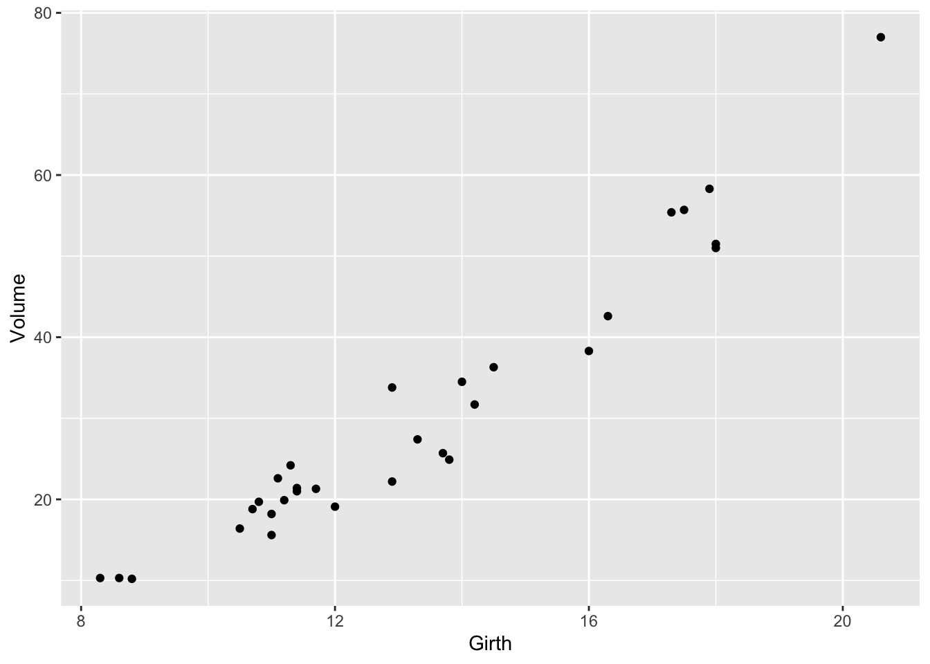
Figure 1: Volume against Girth for black cherry trees
Exercise 28 What happens if you replace geom_point with geom_line?
Exercise 29 And what happens if you add both geoms to the gp object?
The available geoms are documented at http://docs.ggplot2.org/current/.
Windows
By default plots are printed to the Plots window in the bottom right pane of RStudio. To create a new graphics window use the
windows() function, where by default the width and height are both 7 inches. If working with the Mac or Linux Operating systems use the quartz() or X11() function, respectively.
The most recent ggplot object to have been created or modified or plotted can be saved in the working
directory using the ggsave function.
For example to save it as a 4 by 4 inch 600 dots per inch (dpi) Portable Network Graphics (png) file
called trees type ggsave("trees.png",width=4,height=4,dpi=600). 600 dpi png files are recommended for inclusion in word documents.
If the number of open windows becomes unwieldy the command graphics.off() can be used to close all the graphics windows.
Scales
Whereas geoms define the method for representing relationships between data, scales control the mapping from data to visual properties such as colour, shape, position and size. These visual properties are referred to as aesthetics.
For example consider the msleep dataset in the ggplot2 library.
gp <- ggplot(data = msleep, aes(x = bodywt, y = brainwt, size = sleep_total,
    colour = vore))
gp <- gp + geom_point()
gp <- gp + scale_x_continuous(name = "Body Weight (kg)", trans = "log10")
gp <- gp + scale_y_continuous(name = "Brain Weight (kg)", trans = "log10")
gp <- gp + scale_size_continuous(name = "Sleep (hr)")
gp <- gp + scale_color_discrete(name = "Diet")
gp
## Warning: Removed 27 rows containing missing values (geom_point).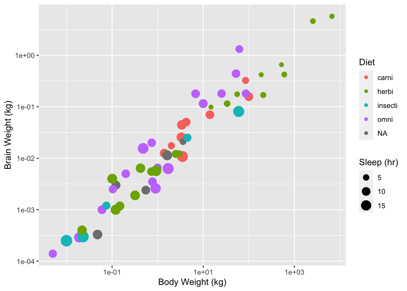
Figure 2: Body weight against brain weight for various mammal species
The above code overides the default positional scales for the x and y data with log10 scales and provides meaningful names. The following code replaces the default discrete color scale with manual values where the color is matched to the diet type.
gp <- gp + scale_colour_manual(name = "Diet", values = c(carni = "red",
    herbi = "green3", omni = "brown", insecti = "black"))
## Scale for 'colour' is already present. Adding another scale for 'colour',
## which will replace the existing scale.Exercise 30 Create a new script called ToothGrowth.R and produce a plot of the ToothGrowth data for inclusion in a word report.
The following ggplot2 functions might be helpful.
geom_jitter(position = position_jitter(width = 0.1))## geom_point: na.rm = FALSE
## stat_identity: na.rm = FALSE
## position_jitterexpand_limits(x = c(0, 2.5))## mapping: x = ~x
## geom_blank: na.rm = FALSE
## stat_identity: na.rm = FALSE
## position_identityFacets
One of the most powerful features of the ggplot2 package is its ability to facet plots. As an example consider the following plot. What does it suggest to you about the relationship between diet and sleep?
gp <- ggplot(data = msleep, aes(x = bodywt, y = brainwt, size = sleep_total))
gp <- gp + facet_grid(. ~ vore)
gp <- gp + geom_point()
gp <- gp + scale_x_continuous(name = "Body Weight (kg)", trans = "log10")
gp <- gp + scale_y_continuous(name = "Brain Weight (kg)", trans = "log10")
gp <- gp + scale_size_continuous(name = "Sleep (hr)")
print(gp)
## Warning: Removed 27 rows containing missing values (geom_point).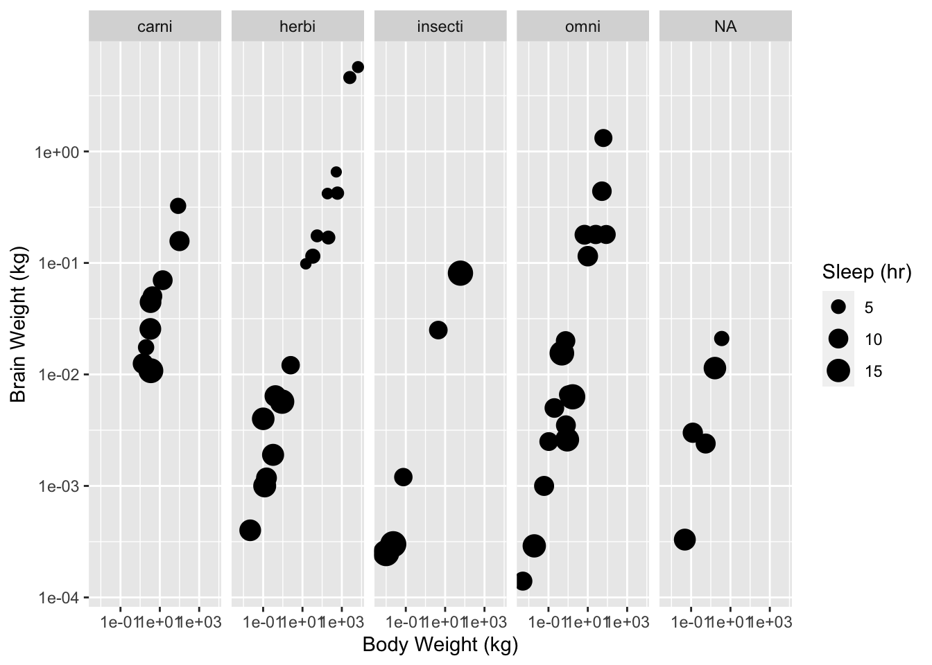
Figure 3: Body weight against brain weight by diet for various mammal species.
Exercise 31 Modify your ToothGrowth.R script so that it produces a second plot facetted by supp.
Themes
The appearance of non-data elements in a ggplot plot is controlled by the theme system. To see the settings for the current theme type . To globally change to the black and white theme use the following code:
theme_set(theme_bw())Alternatively theme parameters can be set for specific ggplot objects using the function. The following code modifies the theme for the current object so that grid lines are not plotted
gp <- gp + theme(panel.grid.major = element_blank(), panel.grid.minor = element_blank())Exercise 32 Alter your ToothGrowth.R script so that it produces a third plot using the black and white theme without grid lines.
Linear Models
Linear regression
The basic linear regression model can be expressed as \[ y_{i} = \alpha +\beta x_{i} + \epsilon_{i} \] where \(\alpha\) is the intercept and \(\beta\) is the slope and the error terms (\(\epsilon_{i}\)) are independent and normally distributed with equal variance.
The following code fits the basic linear regression model where Volume is the response and Girth is the predictor for the trees data set and prints a summary of the model.
mod <- lm(Volume ~ Girth, data = trees)
summary(mod)
##
## Call:
## lm(formula = Volume ~ Girth, data = trees)
##
## Residuals:
## Min 1Q Median 3Q Max
## -8.065 -3.107 0.152 3.495 9.587
##
## Coefficients:
## Estimate Std. Error t value Pr(>|t|)
## (Intercept) -36.9435 3.3651 -10.98 7.62e-12 ***
## Girth 5.0659 0.2474 20.48 < 2e-16 ***
## ---
## Signif. codes: 0 '***' 0.001 '**' 0.01 '*' 0.05 '.' 0.1 ' ' 1
##
## Residual standard error: 4.252 on 29 degrees of freedom
## Multiple R-squared: 0.9353, Adjusted R-squared: 0.9331
## F-statistic: 419.4 on 1 and 29 DF, p-value: < 2.2e-16The model sumary indicates (among other things) that the intercept is -36.9 and the slope is 5.1.
Fitted values
A general approach for plotting the fitted values for any model is to
generate the predicted values for a new data set that covers the range of values of interest and then add them to the plot. New data sets can be easily generated using the new_data function of the newdata package.
library(newdata)
newdata <- new_data(trees, "Girth")
newdata$Volume <- predict(mod, newdata = newdata)

gp <- ggplot(data = trees, aes(x = Girth, y = Volume))
gp <- gp + geom_point()
gp <- gp + geom_line(data = newdata)
print(gp)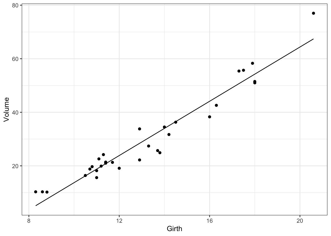
Figure 4: Estimated relationship between Volume and Girth for black cherry trees.
Exercise 33 Step through the above code line by line and document what each line is doing.
Confidence intervals
95% confidence intervals can added to the plot using the same approach.
pred <- data.frame(predict(mod, newdata, interval = "conf"))
newdata <- cbind(newdata, pred)
gp <- gp + geom_line(data = newdata, aes(y = lwr), linetype = "dashed")
gp <- gp + geom_line(data = newdata, aes(y = upr), linetype = "dashed")
print(gp)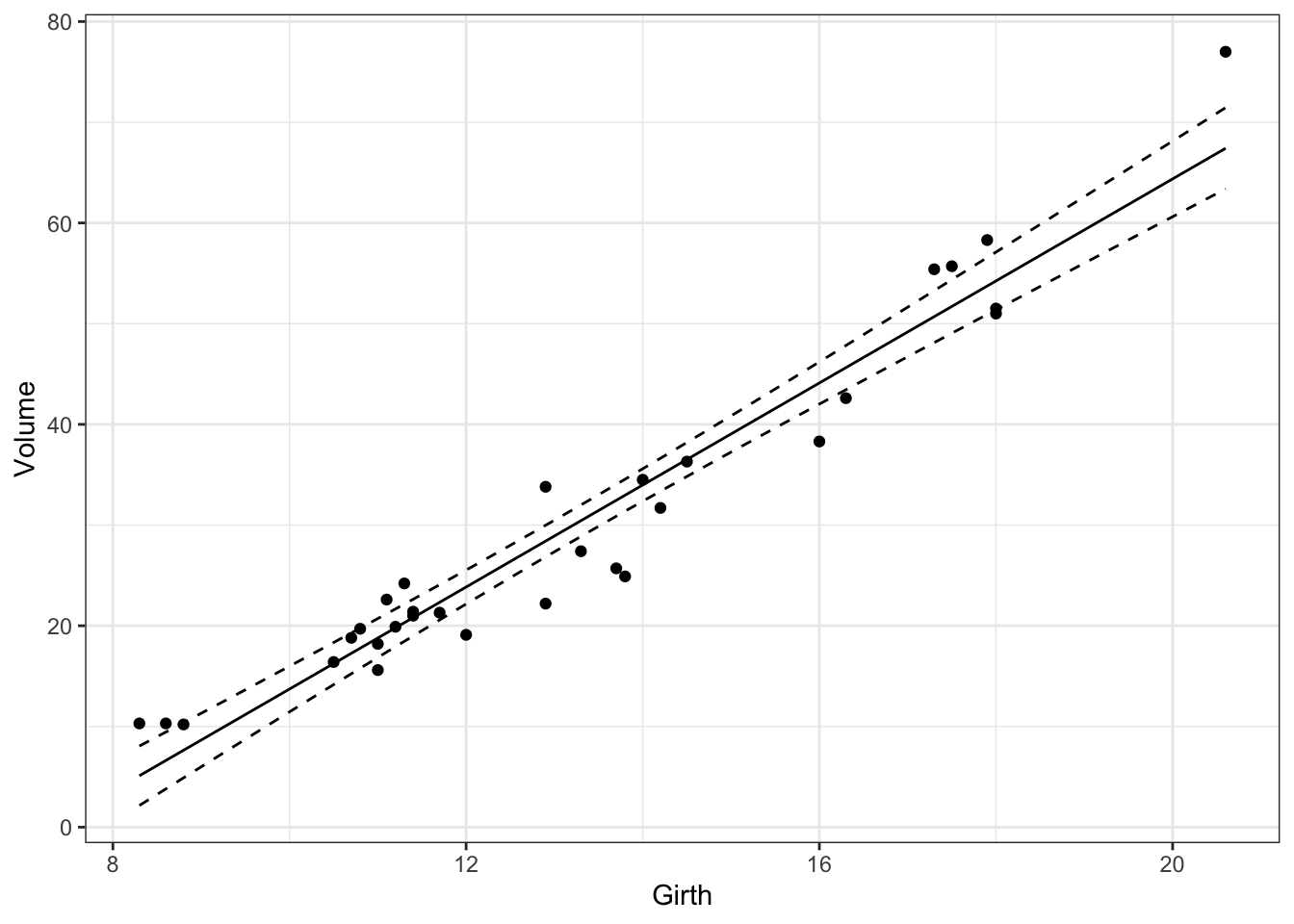
Figure 5: Estimated relationship between Volume and Girth for black cherry trees with 95% confidence intervals.
Prediction intervals
Prediction intervals can be calculated by setting
the interval argument in the predict function to be "pred".
Roughly speaking, confidence intervals represent the uncertainty surrounding the underlying relationship whereas prediction intervals represent the uncertainty surrounding new individual observations.
Exercise 34 Modify your trees.R script so that it fits a linear model to Volume against Girth and plots the observed data with
confidence and prediction intervals.
Model Fit
A linear regression model is only valid if its residuals are consistent with the assumed error structure. A diagnostic plot can be produced using the following code.
qplot(.fitted, .stdresid, data = mod) + geom_hline(yintercept = 0) + geom_smooth(se = FALSE)## `geom_smooth()` using method = 'loess' and formula 'y ~ x'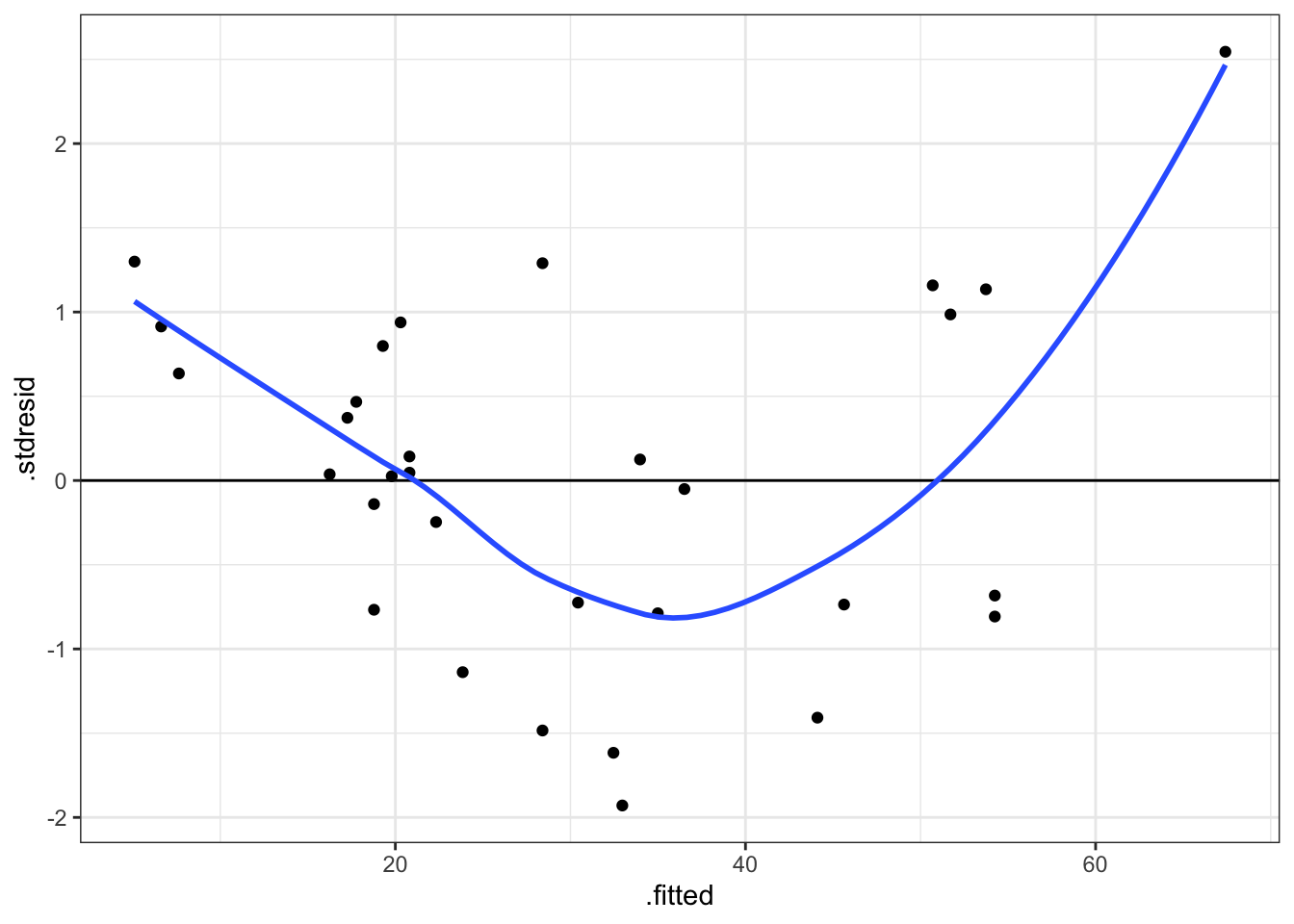
Figure 6: Standardised residuals against fitted values for model of Volume against Girth for black cherry trees.
Exercise 35 What does the previous diagnostic plot suggest to you?
The previous code works because the fortify function has been defined for lm objects. For further examples of diagnostic plots see http://docs.ggplot2.org/current/fortify.lm.html.
The relationship between Volume and Girth is expected to be allometric because the cross-sectional area at an given point scales to the square of the girth (circumference).
Exercise 36 Try fitting an allometric relationship by log transforming
Volume and Girth and then using the same basic linear regression model.
Does the diagnostic plot suggest an improvement in
the model?
ANCOVA
The basic ANCOVA (analysis of covariance) model includes one categorical and one continous predictor variable without interactions. It can be expressed algebraically as follows \[ y_{ij} = \alpha_{i} + \beta x_{j} + \epsilon_{ij}\] where \(\alpha_{i}\) is the intercept for the \(i_{th}\) group mean and \(\beta\) is the slope and the error terms (\(\epsilon_{ij}\)) are independent and normally distributed with equal variance.
The following code fits the basic ANCOVA model to the ToothGrowth data and prints a summary table.
mod <- lm(len ~ supp + dose, data = ToothGrowth)
summary(mod)
##
## Call:
## lm(formula = len ~ supp + dose, data = ToothGrowth)
##
## Residuals:
## Min 1Q Median 3Q Max
## -6.600 -3.700 0.373 2.116 8.800
##
## Coefficients:
## Estimate Std. Error t value Pr(>|t|)
## (Intercept) 9.2725 1.2824 7.231 1.31e-09 ***
## suppVC -3.7000 1.0936 -3.383 0.0013 **
## dose 9.7636 0.8768 11.135 6.31e-16 ***
## ---
## Signif. codes: 0 '***' 0.001 '**' 0.01 '*' 0.05 '.' 0.1 ' ' 1
##
## Residual standard error: 4.236 on 57 degrees of freedom
## Multiple R-squared: 0.7038, Adjusted R-squared: 0.6934
## F-statistic: 67.72 on 2 and 57 DF, p-value: 8.716e-16The model’s coefficients indicate that the slope of the line is 9.3 and that VC is 3.7 less than OJ.
Exercise 37 Are the model’s residuals consistent with the assumed error structure?
The fitted values for both levels of supp can be added to the scatterplot of
len against dose using the same general approach as for the tree data set.
newdata <- new_data(ToothGrowth, c("dose", "supp"))
newdata$len <- predict(mod, newdata = newdata)

gp <- ggplot(data = ToothGrowth, aes(x = dose, y = len, colour = supp))
gp <- gp + geom_point(position = position_jitter(width = 0.1))
gp <- gp + geom_line(data = newdata, aes(group = supp))
print(gp)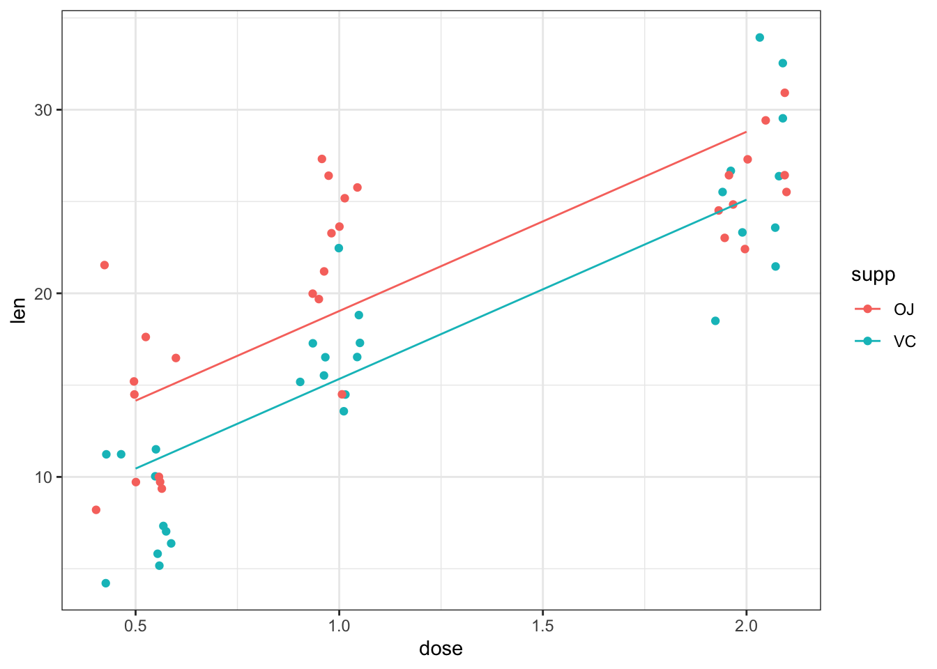
Figure 7: Estimated relationship between tooth length, dose and supplement for guinea pigs fed Vitamin C.
Exercise 38 Modify your script so that it adds the predicted line for both levels of supp to the scatter plot of the ToothGrowth data using the previous code.
The following code fits three additional models corresponding to the ANOVA model with just supp, the linear regression model with just dose and the ANCOVA model with an interaction between dose and supp.
mod2 <- lm(len ~ supp, data = ToothGrowth)
mod3 <- lm(len ~ dose, data = ToothGrowth)
mod4 <- lm(len ~ dose * supp, data = ToothGrowth)
Exercise 39 Modify your script so that it fits all four competing models and then each model’s predictions (along with the raw data) in separate windows.
Exercise 40 Which model provides the best fit to the data?
Functions you might find useful are anova and AIC.
Model Formulae and Functions
This section lists the various functions and formulae required to fit a range of linear, generalized linear, generalized additive, and generalized additive mixed models.
lm(y~1) # one sample t-test
lm(y~x) # basic linear regression
lm(y~fac) # one-way ANOVA
lm(y~x-1) # basic linear regression through the origin (with no intercept term)
lm(y~x+I(x^2)) # polynomial (quadratic) regression
lm(y~x1+x2) # multiple regression
lm(y~x1+x2+x1:x2) # multiple regression with interaction
lm(y~fac1+fac2) # two-way ANOVA
lm(y~x1+fac2) # ANCOVA
nlme::lme(y~x1,random=~1|fac) # linear mixed model
glm(y~x1,family=binomial) # logistic regression
mgcv::gam(y~s(x),family=poisson) # generalized additive model
mgcv::gamm(y~s(x),random=~1|fac,family=Gamma) # generalized additive mixed model
Additional Analyses
Exercise 41 Analyse the chickwts data set. To what extent is diet
a predictor of body weight? Represent your model fit graphically.
Exercise 42 Analyse the msleep data set in the ggplot2 package. To what extent are body weight and diet predictors of brain weight? Are carnivores brainier than herbivores?
R Course Cheat Sheet
| Operator | Description |
|---|---|
- |
Subtraction. Usage: x - y |
; |
Separate lines. Usage: x <- 1; y <- 2 |
:: |
Specify package of object. Usage: datasets::trees |
?? |
Search help files. Usage: ??topic |
? |
Help file. Usage: ?function_name |
( |
Bracket. Usage: x*(y+z) |
* |
Multiplication. Usage: x * y |
/ |
Division. Usage: x / y |
^ |
Power. Usage: x^y |
+ |
Addition. Usage: x + y |
<- |
Assignment. Shortcut: alt-. Usage: x <- y |
$ |
Reference column in data.frame. Useage: x$y |
magrittr::%>% |
Forward pipe operations. Useage: x %>% sum() |
| Math Function | Description |
|---|---|
cumsum |
Cumulative sum. Usage: cumsum(x) |
exp |
Exponential. Usage: exp(x) |
log |
Logarithm. Usage: log(x, base = 10) |
mean |
Average. Usage: mean(x, na.rm = TRUE) |
sqrt |
Square-root. Usage: sqrt(x) |
| Vector Function | Description |
|---|---|
as.factor |
Coerce to factor. Useage: as.factor(x) |
as.numeric |
Coerce to numeric. Useage: as.factor(x) |
c |
Concatenate. Usage: c(1, -3, 5) |
length |
Length. Usage: length(seq(2, 5)) |
seq |
Sequence. Usage: seq(1, 4) |
| data.frame Function | Description |
|---|---|
cbind |
Combine two data.frames by columns. |
data.frame |
Create data.frame. |
data |
List available data sets. |
newdata::new_data |
Dummy data set. |
dplyr::arrange |
Sort rows. |
dplyr::filter |
Chose a subset of rows based on conditions. |
dplyr::mutate |
Add new columns. |
dplyr::select |
Chose a subset of columns based on names. |
head |
Chose first six rows. |
na.omit |
Delete missing values. |
read.csv |
Input from csv file. |
tidyr::gather |
Convert from wide to long format |
tidyr::spread |
Convert from long to wide format |
write.csv |
Output as csv file. |
| Graphics Function | Description |
|---|---|
ggplot2::element_blank |
Blank value for a theme element. |
ggplot2::expand_limits |
Expand scale limits to include specified values. |
ggplot2::facet_grid |
Break plot into facets by variables. |
ggplot2::geom_hline |
Represent values with horizontal lines. |
ggplot2::geom_jitter |
Represent values with points plus random spread. |
ggplot2::geom_line |
Represent values with lines. |
ggplot2::geom_point |
Represent values with points. |
ggplot2::geom_smooth |
Represent values with smoothers. |
ggplot2::ggplot |
Set data.frame and aesthetic mappings for ggplot graphic object. |
ggplot2::ggsave |
Save current plot. |
ggplot2::qplot |
Quick wrapper for ggplot and geom_point. |
ggplot2::scale_color_discrete |
Set discrete color scale attributes. |
ggplot2::scale_color_manual |
Set manual color scale attributes. |
ggplot2::scale_size_continuous |
Set continuous size scale attributes. |
ggplot2::scale_x_continuous |
Set continuous x position scale attributes. |
ggplot2::scale_y_continuous |
Set continuous y position scale attributes. |
ggplot2::theme_get |
Get current theme for graphics. |
ggplot2::theme_set |
Set current theme for graphics. |
ggplot2::theme |
Set theme element for current graphic object. |
graphics.off |
Close all graphics windows. |
windows |
New graphics window. Use quartz() or X11() for OSX or linux |
| Model Function | Description |
|---|---|
AIC |
Akaike’s Information Criterion for one or more models. |
anova |
Analysis of variance tables for one or more models. |
lm |
Fit linear model. Useage: lm(y ~ x, data = data) |
predict |
Predict response values for model. |
| General Function | Description |
|---|---|
class |
Class of object. Usage: class(x) |
devtools::install_github |
Install package from GitHub. |
getwd |
Get working directory. Useage: getwd(). |
install.packages |
Install package(s) from CRAN. Useage: install.packages('pkg_name') |
library |
Load installed package. Useage: library(package_name) |
ls |
Objects in workspace or package. Usage: ls(); ls(2) |
print |
Print to console or draw graphics object in window |
rm |
Remove object(s) from workspace. Usage: rm(x); rm(list = ls()) |
search |
Loaded packages. Useage: search() |
setwd |
Set working directory. Useage: setwd('path_to_dir') |
summary |
Summary of object. Useage: summary(x) |