Quesnel Exploitation Analysis 2022
The suggested citation for this analytic appendix is:
Dalgarno, S. & Thorley, J.L. (2023) Quesnel Exploitation Analysis 2022. A Poisson Consulting Analytic Appendix. URL: https://www.poissonconsulting.ca/f/1230088647.
Background
Quesnel Lake supports a recreational fishery for Rainbow Trout. To provide information on the natural and fishing mortality, Rainbow Trout were caught by angling and tagged with acoustic transmitters and/or a $100 and $10 reward tag.
The objectives of this analysis are to:
- Provide a complete history of tagged fish from capture to tag expiry
and estimated fate.
- Provide a summary of life history including variation in fork length
at spawning under different lake conditions and any additional
observations on change in population age structure and size.
- Estimate annual in-lake abundance >= 50 cm from mark-recapture data
in years with sufficient data.
- Provide an assessment of conservation impacts and allowable exploitation if changing the lower slot limit to 60 cm or 70 cm.
Data Preparation
The outing, receiver deployment, detection, fish capture and recapture information were provided by the Ministry of Forests, Lands and Natural Resource Operations and added to a SQLite database.
The data were prepared for analysis using R version 4.3.0 (R Core Team 2022).
Receivers were assumed to have a detection range of 500 m. Detections were aggregated daily, where for each transmitter the receiver with the most number of detections was chosen. In the case of a tie, the receiver with the greatest coverage area was chosen. Only individuals with a fork length (FL) \(\geq\) 450 mm, an acoustic tag life \(\geq\) 365 days (if acoustically tagged) and a $100 and $10 reward tags were included in the survival analysis.
Statistical Analysis
Model parameters were estimated using Bayesian methods. The estimates were produced using JAGS (Plummer 2003). For additional information on Bayesian estimation the reader is referred to McElreath (2020).
Unless stated otherwise, the Bayesian analyses used weakly informative normal and half-normal prior distributions (Gelman, Simpson, and Betancourt 2017). The posterior distributions were estimated from 1500 Markov Chain Monte Carlo (MCMC) samples thinned from the second halves of 3 chains (Kery and Schaub 2011, 38–40). Model convergence was confirmed by ensuring that the potential scale reduction factor \(\hat{R} \leq 1.05\) (Kery and Schaub 2011, 40) and the effective sample size (Brooks et al. 2011) \(\textrm{ESS} \geq 150\) for each of the monitored parameters (Kery and Schaub 2011, 61).
The parameters are summarised in terms of the point estimate, lower and upper 95% credible limits (CLs) and the surprisal s-value (Greenland 2019). The estimate is the median (50th percentile) of the MCMC samples while the 95% CLs are the 2.5th and 97.5th percentiles. The s-value indicates how surprising it would be to discover that the true value of the parameter is in the opposite direction to the estimate (Greenland 2019). An s-value of \(>\) 4.3 bits, which is equivalent to a significant p-value \(<\) 0.05 (Kery and Schaub 2011; Greenland and Poole 2013), indicates that the surprise would be equivalent to throwing at least 4.3 heads in a row.
The condition that parameters describing the effects of secondary (nuisance) explanatory variable(s) have significant p-values was used as a model selection heuristic (Kery and Schaub 2011). Based on a similar argument, the condition that random effects have a standard deviation with a lower 95% CL \(>\) 5% of the estimate was used as an additional model selection heuristic. Primary explanatory variables are evaluated based on their estimated effect sizes with 95% CLs (Bradford, Korman, and Higgins 2005)
Where possible, model adequacy was assessed via posterior predictive checks (Kery and Schaub 2011). More specifically, the number of zeros and the first four central moments (mean, variance, skewness and kurtosis) for the deviance residuals were compared to the expected values by simulating new residuals. In this context the s-value indicates how surprising each observed metric is given the estimated posterior probability distribution for the residual variation.
The results are displayed graphically by plotting the modeled relationships between particular variables and the response(s) with the remaining variables held constant. In general, continuous and discrete fixed variables are held constant at their mean and first level values, respectively, while random variables are held constant at their typical values (expected values of the underlying hyperdistributions) (Kery and Schaub 2011, 77–82).
The analyses were implemented using R version 4.3.0
(R Core Team 2022) and the
mbr family of packages.
Model Descriptions
Condition
The expected weight of fish of a given length were estimated from the data using a mass-length model (He et al. 2008).
More specifically the model was based on the allometric relationship
\[ W = \alpha L^{\beta}\]
where \(W\) is the weight (mass), \(\alpha\) is the coefficent, \(\beta\) is the exponent and \(L\) is the length.
To improve chain mixing the relation was log-transformed, i.e.,
\[ \log(W) = \log(\alpha) + \beta \cdot \log(L)\] Length and weights of fish were taken from two sources: captures from broodstock collection in the Horsefly River (2015-2022) and in-lake captures from tagging outings (2013-2022).
Key assumptions of the condition model include:
- The expected weight is allowed to vary with length and date.
- The expected weight is allowed to vary randomly with year and source within year.
- The relationship between weight and length is allowed to vary with date.
- The residual variation in weight is log-normally distributed.
Growth
Annual growth of fish were estimated from inter-annual recaptures (in-lake and broodstock) and aged broodstock captures using the Fabens method (Fabens 1965) for estimating the von Bertalanffy growth curve (von Bertalanffy 1938). This curve is based on the premise that:
\[ \frac{\text{d}L}{\text{d}t} = k (L_{\infty} - L)\]
where \(L\) is the length of the individual, \(k\) is the growth coefficient and \(L_{\infty}\) is the maximum length.
Integrating the above equation gives:
\[ L_t = L_{\infty} (1 - e^{-k(t - t_0)})\]
where \(L_t\) is the length at time \(t\) and \(t_0\) is the time at which the individual would have had zero length.
The Fabens form allows
\[ L_r = L_c + (L_{\infty} - L_c) (1 - e^{-kT})\]
where \(L_r\) is the length at recapture, \(L_c\) is the length at capture and \(T\) is the time between capture and recapture.
For aged fish, length at capture is the length at Age-0 \(L_0\), estimated
with the modified form:
\[L_r = L_{0} - (L_{\infty} - L_0) (1 - e^{-kA})\] where \(A\) is the age.
Key assumptions of the growth model include:
- The mean maximum length \(L_{\infty}\) is constant.
- The growth coefficient \(k\) varies randomly with growth year.
- \(L_{\infty}\) is likely between 800 and 1000.
- The residual variation in growth is student-t distributed.
- The student-t shape parameter is fixed at 2.
A growth year spans April 01 to March 31 the following year.
Preliminary analyses indicated lack of support for variation in \(k\) by Horsefly River sockeye run size with a one or two year lag.
Survival
The natural mortality and recapture probability were estimated using a Bayesian individual state-space survival model (Thorley and Andrusak 2017) with three month intervals. The survival model incorporated natural and handling mortality, acoustic detections, inter-section movement, T-bar tag loss, spawning, recapture, reporting, fork length at spawning and sockeye run size in the previous year.
T-bar tag loss was estimated from the number of tags reported from recaught double-tagged individuals (Fabrizio et al. 1999). The model assumes that tag loss is not a time-dependent process and occurs following initial release.
Fork length at spawning was calculated from the measured length at capture (\(L_{i,fi}\)) plus the length increment expected under a Von Bertalanffy Growth Curve (Walters & Martell, 2004)
\[L_{i,t} = L_{i,fi} + (L_{∞} − L_{i,fi} )(1 − e^{(−0.25 \cdot k(t −fi))})\]
where the 0.25 in the exponent adjusts for the fact that there are four time periods per year. Values for \(L_\infty\) and annual \(k\) and were estimated in the growth model.
The probability of spawning at estimated length \(L\) is determined by
\[S = \frac{L^{S_p}}{L_s^{S_p} + L^{S_p}} \cdot es\]
where \(L_s\) is the length at which 50% of fish are mature, \(es\) is the probability of a mature fish spawning and \(S_p\) is the maturity (as a function of length) power.
Key assumptions of the spawning probability sub-model include:
- \(L_s\) varies randomly by year
- \(es\) varies randomly by year
A fish was considered to have spawned in a given year if one of the following conditions were met: detected within a spawning river during the spawning period with a detection hiatus (no detections in lake) of at least 7 days; or detected within a spawning gate during the spawning period with a detection hiatus of at least 14 days. Cutoff values for minimum hiatus periods were determined by inspecting the distribution of in-lake hiatus periods for fish detected in spawning rivers and the distribution of all hiatus periods for suspected spawners within the spawning period.
In addition to assumptions 1 to 2 and 4 to 10, in Thorley and Andrusak (2017), the model also assumes that:
- The natural mortality varies by season, spawning and sockeye
abundance for each size class.
- The recapture probability varies randomly by year.
- The recapture probability varies by season.
- The probability of tag loss is independent between tags on a fish.
- The probability of detection depends on whether a fish is alive or has died near or far from a receiver
- All recaptured fish that are released have their FLOY tags removed.
- Reporting of recaptured fish with one or more T-bar tags is likely greater than 90%.
Seasons are defined as winter (January to March), spring (April to June), summer (July to September), and fall (October to December).
Size classes are defined as small (\(\le\) 600 mm), medium (601 \(-\) 700 mm) and large (\(>\) 700 mm).
Sockeye abundance is the Horsefly River run size with a two year lag (i.e., spawning in the spring of 2016 is associated with autumn 2014 sockeye abundance).
Preliminary analyses indicated lack of support for variation in mortality by year, sockeye year (October 01 to September 30 the following year) and size class within year.
Mark-Recapture
The in-lake and spawner abundance for individuals \(\ge\) 500 mm were estimated using hierarchical Bayesian mark-recapture sub-models within the survival model, where the number of alive marked individuals in the lake at each time period was estimated from the ‘Alive’ latent state in the previous period. The number of spawning marked individuals was estimated from the spawning probability and the number of alive marked individuals in the previous period.
The ‘in-lake’ mark-recapture model estimated abundance from in-lake captures and recaptures from researcher tagging outings.
The ‘spawner’ mark-recapture model estimated spawner abundance from spawner captures and recaptures from broodstock collection in the Horsefly River.
An additional in-lake abundance \(A_L\) estimate was derived from estimated spawner abundance \(A_S\) and spawning probability \(P_S\) given the following: \[A_L = \frac{A_S}{P_S} \]
Key assumptions of the mark-recapture models include:
- Marked fish mix randomly with unmarked fish within the lake.
- The probability of capturing a marked or unmarked fish is the same.
- All recaptured fish are correctly identified as being marked.
- The number of recaptures (of fish marked at that site in that year) and the total number of fish caught are each binomially distributed.
Additional assumptions for the lake model include:
- Capture efficiency varies by total outing hours in a three month
period.
- Abundance varies randomly by year.
Yield-Per-Recruit
The optimal yield (defined as the harvested number of fish as percent of the number of recruits at carrying capacity) was calculated using a yield-per-recruit approach (Bison, O’Brien, and Martell 2003).
Scenarios explored include:
- Lower slot limit (
Llo) of 40, 50, 60, 70, 80 and 90, with other YPR parameter values held constant.
Rk(lifetime spawners per spawner at low density) values of 5, 7.5, and 10 andLs(length at 50% mature) values of 55, 60, and 65, withLloheld at 60.
Rkvalues of 5, 7.5, and 10 andLsvalues of 55, 60, and 65, withLloheld at 50.
Key assumptions include:
- The population is at equilibrium.
- All captured individuals above
Lloare retained. - All captured individuals below
Lloare released. - Handling mortality is 10%.
- The life-history parameters are fixed.
- There are no Allee effects.
- There are no limitations on prey species.
Model Templates
Condition
.model{
  bWeight ~ dnorm(3, 2^-2)
  bWeightLength ~ dnorm(3, 1^-2)
  bWeightDayte ~ dnorm(0, 1^-2);
  bWeightLengthDayte ~ dnorm(0, 1^-2)
  sWeightAnnual ~ dexp(1)
  for(i in 1:nAnnual) {
    bWeightAnnual[i] ~ dnorm(0, sWeightAnnual^-2)
  }
  sWeightSourceAnnual ~ dexp(1)
  for(i in 1:nSource){
    for(j in 1:nAnnual){
      bWeightSourceAnnual[i,j] ~ dnorm(0, sWeightSourceAnnual^-2)
    }
  }
  sWeight ~ dexp(1)
  for(i in 1:nObs) {
    log(eWeight[i]) <- bWeight + bWeightDayte * Dayte[i] + bWeightAnnual[Annual[i]] + bWeightSourceAnnual[Source[i], Annual[i]] + (bWeightLength + bWeightLengthDayte * Dayte[i]) * (log(Length[i]) - log(100))
    Weight[i] ~ dlnorm(log(eWeight[i]), sWeight^-2)
  }
Block 1. Model description.
Growth
.model {
  bK ~ dnorm(0, 2^-2)
  bL0 ~ dnorm(0, 100^-2)
  sKYear ~ dexp(1)
  theta <- 0.5

  bLinf ~ dnorm(900, 100^-2) T(0,)
  sGrowth ~ dexp(1)
  sLength ~ dexp(1)
  for (i in 1:nYear) {
    bKYear[i] ~ dnorm(0, sKYear^-2)
    log(eK[i]) <- bK + bKYear[i]
  }
  for(i in 1:nAged){
    eLength[i] <- bLinf - (bLinf - bL0) * exp(-exp(bK) * Age[i])
    Length[i] ~ dnorm(eLength[i], sLength^-2)
  }
  for(i in 1:nFish){
    eL0[i] <- max(bL0, LengthAtRelease[i])
    for(j in 1:nYear){
      ekProp[i,j] <- eK[j] * pYear[i,j]
    }
    eSumEk[i] <- exp(-sum(ekProp[i,]))
    eGrowth[i] <- max(0, (bLinf - eL0[i]) * (1 -eSumEk[i]))
    Growth[i] ~ dt(eGrowth[i], sGrowth^-2, 1/theta)
  }
Block 2.
Tag Loss
model {
  bTagLoss ~ dbeta(1, 1)

  for (i in 1:nObs) {
    TagsRecap[i] ~ dbin(1 - bTagLoss, 2) T(1,)
  }
Block 3. Model description.
Survival
.model{
  bMortality ~ dnorm(-3, 3^-2)
  bMortalitySpawning ~ dnorm(0, 2^-2)
  bLs ~  dnorm(6, 2^-2)
  bSp ~ dexp(1/20)
  bEs ~ dnorm(0, 2^-2)

  bDetectedAlive ~ dbeta(1, 1)
  bDieNear ~ dbeta(1, 1)
  bDetectedDeadNear ~ dbeta(10, 1)
  bDetectedDeadFar ~ dbeta(1, 10)
  bMoved ~ dbeta(1, 1)
  bRecaptured ~ dnorm(0, 2^-2)
  bReported ~ dbeta(10, 1)
  bReleased ~ dbeta(1, 1)
  bReleasedResearcher ~ dbeta(1, 1)
  bRecapturedResearcher ~ dbeta(5, 1)
  bTagLoss <- 0.0545
  bTagLossT <- 0.0001

  bEfficiency ~ dnorm(-4, 2^-2)
  bAbundance ~ dnorm(7, 2^-2)
  bOutingHours ~ dnorm(0, 2^-2)
  bEfficiencySpawn ~ dnorm(-4, 2^-2)
  bAbundanceSpawn ~ dnorm(1000, 500^-2)

  bMortalitySeason[1] <- 0
  for (i in 2:nSeason) {
    bMortalitySeason[i] ~ dnorm(0, 2^-2)
  }
  for (i in 1:nSizeClass) {
    bMortalitySockeye[i] ~ dnorm(0, 2^-2)
  }
  sRecapturedAnnual ~ dexp(1)
  for (i in 1:nAnnual) {
    bRecapturedAnnual[i] ~ dnorm(0, sRecapturedAnnual^-2)
  }
  bRecapturedSeason[1] <- 0
  for (i in 2:nSeason) {
    bRecapturedSeason[i] ~ dnorm(0, 2^-2)
  }
  sLsAnnual ~ dexp(1)
  for (i in 1:nAnnual) {
    bLsAnnual[i] ~ dnorm(0, sLsAnnual^-2)
  }
  sEsAnnual ~ dexp(1)
  for (i in 1:nAnnual) {
    bEsAnnual[i] ~ dnorm(0, sEsAnnual^-2)
  }

  for (i in 1:nCapture){
    eDetectedAlive[i] <- bDetectedAlive
    eDieNear[i] ~ dbern(bDieNear)
    eDetectedDeadNear[i] <- bDetectedDeadNear
    eDetectedDeadFar[i] <- bDetectedDeadFar
    eDetectedDead[i] <- eDieNear[i] * eDetectedDeadNear[i] + (1 - eDieNear[i]) * eDetectedDeadFar[i]

    logit(eMortality[i,PeriodCapture[i]]) <- bMortality + bMortalitySeason[Season[PeriodCapture[i]]] + bMortalitySockeye[SizeClass[i,PeriodCapture[i]]] * SockeyePrevious[PeriodCapture[i]]
    logit(eRecaptured[i,PeriodCapture[i]]) <- bRecaptured + bRecapturedSeason[Season[PeriodCapture[i]]] + bRecapturedAnnual[Annual[PeriodCapture[i]]]

    eMoved[i,PeriodCapture[i]] <- bMoved
    eReported[i,PeriodCapture[i]] <- bReported
    eReleased[i,PeriodCapture[i]] <- bReleased
    eReleasedResearcher[i,PeriodCapture[i]] <- bReleasedResearcher
    eRecapturedResearcher[i,PeriodCapture[i]] <- bRecapturedResearcher

    InLake[i,PeriodCapture[i]] <- 1
    Alive[i,PeriodCapture[i]] ~ dbern(1-eMortality[i,PeriodCapture[i]])
    Alive50[i,PeriodCapture[i]] <- Alive[i,PeriodCapture[i]] * (Length[i,PeriodCapture[i]] >= 500)

    TBarTag100[i,PeriodCapture[i]] ~ dbern(1-bTagLoss)
    TBarTag10[i,PeriodCapture[i]] ~ dbern(1-bTagLoss)

    eDetected[i,PeriodCapture[i]] <- Alive[i,PeriodCapture[i]] * eDetectedAlive[i] + (1-Alive[i,PeriodCapture[i]]) * eDetectedDead[i]
    Detected[i,PeriodCapture[i]] ~ dbern(Monitored[i,PeriodCapture[i]] * eDetected[i,PeriodCapture[i]])
    Moved[i,PeriodCapture[i]] ~ dbern(Alive[i,PeriodCapture[i]] * Detected[i,PeriodCapture[i]] * eMoved[i,PeriodCapture[i]])

    RecapturedResearcher[i,PeriodCapture[i]] ~ dbern(Alive[i,PeriodCapture[i]] * eRecapturedResearcher[i,PeriodCapture[i]])
    Recaptured[i,PeriodCapture[i]] ~ dbern(Alive[i,PeriodCapture[i]] * eRecaptured[i,PeriodCapture[i]])
    Reported[i,PeriodCapture[i]] ~ dbern(Recaptured[i,PeriodCapture[i]] * eReported[i,PeriodCapture[i]] * step(TBarTag100[i,PeriodCapture[i]] + TBarTag10[i,PeriodCapture[i]] - 1))
    Released[i,PeriodCapture[i]] ~ dbern(Recaptured[i,PeriodCapture[i]] * eReleased[i,PeriodCapture[i]])
    ReleasedResearcher[i,PeriodCapture[i]] ~ dbern(RecapturedResearcher[i,PeriodCapture[i]] * eReleasedResearcher[i,PeriodCapture[i]])

  for(j in (PeriodCapture[i]+1):nPeriod) {
    log(eLs[i,j]) <- bLs + bLsAnnual[Annual[j]]
    logit(eEs[i,j]) <- bEs + bEsAnnual[Annual[j]]
    eSpawning[i,j] <- (((Length[i,j]^bSp) / (eLs[i,j]^bSp + Length[i,j]^bSp)) * eEs[i,j])
    Spawned[i,j] ~ dbern(Alive[i,j-1] * Monitored[i,j] * SpawningPeriod[j] * eSpawning[i,j])
    logit(eMortality[i,j]) <- bMortality + bMortalitySpawning * Spawned[i,j-1] + bMortalitySeason[Season[j]] + bMortalitySockeye[SizeClass[i,j]] * SockeyePrevious[j]
    logit(eRecaptured[i,j]) <- bRecaptured + bRecapturedSeason[Season[j]] + bRecapturedAnnual[Annual[j]]

    eMoved[i,j] <- bMoved
    eRecapturedResearcher[i,j] <- bRecapturedResearcher
    eReported[i,j] <- bReported
    eReleased[i,j] <- bReleased
    eReleasedResearcher[i,j] <- bReleasedResearcher

    InLake[i,j] ~ dbern(InLake[i,j-1] * ((1 - (Recaptured[i,j-1])) + Recaptured[i,j-1] * Released[i,j-1]) * ((1 - (RecapturedResearcher[i,j-1])) + RecapturedResearcher[i,j-1] * ReleasedResearcher[i,j-1]))
    Alive[i,j] ~ dbern(InLake[i,j] * Alive[i,j-1] * (1-eMortality[i,j]))
    Alive50[i,j] <- Alive[i,j] * (Length[i,j] >= 500)
    TBarTag100[i,j] ~ dbern(TBarTag100[i,j-1] * (1-Recaptured[i,j-1]) * (1-bTagLossT))
    TBarTag10[i,j] ~ dbern(TBarTag10[i,j-1] * (1-Recaptured[i,j-1]) * (1-bTagLossT))

    eDetected[i,j] <- Alive[i,j] * eDetectedAlive[i] + (1-Alive[i,j]) * eDetectedDead[i]
    Detected[i,j] ~ dbern(InLake[i,j] * Monitored[i,j] * eDetected[i,j])
    Moved[i,j] ~ dbern(Alive[i,j] * Detected[i,j] * eMoved[i,j])

    RecapturedResearcher[i,j] ~ dbern(Alive[i,j] * eRecapturedResearcher[i,j] * step(TBarTag100[i,j] + TBarTag10[i,j] - 1))
    Recaptured[i,j] ~ dbern(Alive[i,j] * eRecaptured[i,j])
    Reported[i,j] ~ dbern(Recaptured[i,j] * eReported[i,j] * step(TBarTag100[i,j] + TBarTag10[i,j] - 1))
    Released[i,j] ~ dbern(Recaptured[i,j] * eReleased[i,j])
    ReleasedResearcher[i,j] ~ dbern(RecapturedResearcher[i,j] * eReleasedResearcher[i,j])
  }
  }
  Marked[1] <- sum(Alive50[1:PeriodCaptures[1],1])
  MarkedSpawners[1] <- 1
  for(p in 2:nPeriod){
      Marked[p] <- sum(Alive50[1:PeriodCaptures[p],p])
      logit(eSpawningPeriod[p]) <- bEs + bEsAnnual[Annual[p]]
      MarkedSpawners[p] ~ dpois(Marked[p-1] * eSpawningPeriod[p])
  }
  sAbundanceAnnual ~ dexp(1)
  for (i in 1:nAnnualOuting) {
    bAbundanceAnnual[i] ~ dnorm(0, sAbundanceAnnual^-2)
  }
  eAbundanceSpawn ~ dpois(bAbundanceSpawn)
  for(l in 1:nPeriodCount){
      logit(eEfficiencySpawn[l]) <- bEfficiencySpawn
      RecaptureSpawners[l] ~ dbin(eEfficiencySpawn[l], MarkedSpawners[PeriodCount[l]])
      CaptureSpawners[l] ~ dbin(eEfficiencySpawn[l], eAbundanceSpawn)
  }

  for(k in 1:nPeriodOuting){
      log(eAbundance[k]) <- bAbundance + bAbundanceAnnual[AnnualOuting[k]]
      eAbundanceInt[k] ~ dpois(eAbundance[k])
      logit(eEfficiency[k]) <- bEfficiency + bOutingHours * OutingHours[PeriodOuting[k]]
      Recaptures[k] ~ dbin(eEfficiency[k], Marked[PeriodOuting[k]-1])
      Captures[k] ~ dbin(eEfficiency[k], eAbundanceInt[k])
  }
Block 4. Survival model description.
Results
Tables
Condition
Table 1. Parameter descriptions.
| Parameter | Description |
|---|---|
Annual[i] |
Year the ith fish was captured as a factor |
Dayte[i] |
Day of year that the ith fish was captured |
Length[i] |
Fork length of the ith fish |
Source[i] |
Data source for the ith fish (lake or
broodstock) |
Weight[i] |
Recorded weight of the ith fish |
bWeightAnnual[i] |
Effect of the ith Annual on bWeight |
bWeightDayte[i] |
Effect of the ith Dayte on bWeight |
bWeightLengthDayte[i] |
Effect of the ith Dayte on bWeightLength |
bWeightLength |
Effect of log(Length[i]) on bWeight |
bWeightSourceAnnual[i] |
Effect of the ith Source within the jth
Annual on bWeight |
bWeight |
Intercept of log(eWeight[i]) |
eWeight[i] |
Expected Weight[i] of the ith fish |
sWeightAnnual |
SD of bWeightAnnual |
sWeightSourceAnnual |
SD of bSourceAnnual |
sWeight |
SD of log(Weight[i]) |
Table 2. Model coefficients.
| term | estimate | lower | upper | svalue |
|---|---|---|---|---|
| bWeight | 2.2722775 | 2.1647061 | 2.3739569 | 10.55171 |
| bWeightDayte | -0.2371098 | -0.3462110 | -0.1279576 | 10.55171 |
| bWeightLength | 3.1081631 | 3.0577862 | 3.1634224 | 10.55171 |
| bWeightLengthDayte | 0.1527845 | 0.0930352 | 0.2145596 | 10.55171 |
| sWeight | 0.1086107 | 0.1042768 | 0.1132872 | 10.55171 |
| sWeightAnnual | 0.0455064 | 0.0034942 | 0.1121414 | 10.55171 |
| sWeightSourceAnnual | 0.0616008 | 0.0349995 | 0.1013398 | 10.55171 |
Table 3. Model summary.
| n | K | nchains | niters | nthin | ess | rhat | converged |
|---|---|---|---|---|---|---|---|
| 1124 | 7 | 3 | 500 | 100 | 178 | 1.008 | TRUE |
Table 4. Model posterior predictive checks.
| moment | observed | median | lower | upper | svalue |
|---|---|---|---|---|---|
| zeros | 0.0000000 | 0.0000000 | 0.0000000 | 0.0000000 | 0.0000000 |
| mean | 0.0000426 | -0.0005523 | -0.0619175 | 0.0582786 | 0.0271665 |
| variance | 0.9834447 | 1.0000853 | 0.9184694 | 1.0790217 | 0.5196625 |
| skewness | -0.2243304 | -0.0017212 | -0.1427099 | 0.1503316 | 10.5517083 |
| kurtosis | 0.0653836 | -0.0173751 | -0.2628448 | 0.3158036 | 0.8186929 |
Table 5. Model sensitivity.
| all | analysis | sensitivity | bound |
|---|---|---|---|
| all | 1.008 | 1.015 | 1.013 |
Growth
Table 6. Parameter descriptions.
| Parameter | Description |
|---|---|
Growth[i] |
Observed growth between release and recapture of ith
recapture |
LengthAtRelease[i] |
Length at previous release of ith recapture |
Year[i] |
Release year of ith recapture |
bKYear[i] |
Effect of ith Year on bK |
bK |
Intercept of log(eK) |
bLinf |
Mean maximum length |
eGrowth |
Expected Growth between release and recapture |
eK[i] |
Expected von Bertalanffy growth coefficient for ith
Year |
eSumK[i] |
Expected sum of the proportion of annual von Bertalanffy growth coefficient between release and recapture |
pYear[i] |
Proortion of Years between release and recapture of ith
recapture |
sGrowth |
Log standard deviation of residual variation in Growth |
sKYear |
Log standard deviation of bKYear |
Table 7. Model coefficients.
| term | estimate | lower | upper | svalue |
|---|---|---|---|---|
| bK | -1.4320124 | -1.5455592 | -1.3142231 | 10.551708 |
| bL0 | -20.1326797 | -65.1034093 | 13.9370296 | 1.918713 |
| bLinf | 854.8911464 | 818.6242759 | 894.1474971 | 10.551708 |
| sGrowth | 28.2133323 | 25.2070680 | 32.2250808 | 10.551708 |
| sKYear | 0.4060662 | 0.2429683 | 0.6943251 | 10.551708 |
| sLength | 49.8966766 | 46.1097545 | 54.2918162 | 10.551708 |
Table 8. Model summary.
| n | K | nchains | niters | nthin | ess | rhat | converged |
|---|---|---|---|---|---|---|---|
| 5580 | 6 | 3 | 500 | 30 | 222 | 1.008 | TRUE |
Tag Loss
Table 9. Parameter descriptions.
| Parameter | Description |
|---|---|
TagsRecap[i] |
Tags remaining on ith recapture |
bTagLossIntercept |
Intercept for logit(eTagLoss) |
eTagLoss[i] |
Predicted probability of single tag loss for the ith recapture |
Table 10. Model coefficients.
| term | estimate | lower | upper | svalue |
|---|---|---|---|---|
| bTagLoss | 0.0537979 | 0.0312079 | 0.0862457 | 10.55171 |
Table 11. Model summary.
| n | K | nchains | niters | nthin | ess | rhat | converged |
|---|---|---|---|---|---|---|---|
| 126 | 1 | 3 | 500 | 10 | 1500 | 1 | TRUE |
Table 12. The number of recaptured fish that were reported without their $100 versus $10 reward tag by species.
| Species | Loss100 | Loss10 |
|---|---|---|
| Rainbow Trout | 0 | 11 |
Table 13. Model sensitivity.
| all | analysis | sensitivity | bound |
|---|---|---|---|
| all | 1 | 1 | 1 |
Survival
Table 14. Parameter descriptions.
| Parameter | Description |
|---|---|
TagLossT |
Seasonal probability of loss of a single tag in all periods subsequent to capture |
TagLoss |
Seasonal probability of loss of a single tag in the period of capture |
bAbundanceAnnual |
Effect of ith Year on bAbundance |
bAbundanceSpawn |
Expected spawner abundance |
bAbundance |
Expected in-lake abundance |
bDetectedAlive |
Seasonal probability of detection if in-lake |
bDetectedDeadFar |
Seasonal probability of detection if in-lake and dead far from a receiver |
bDetectedDeadNear |
Seasonal probability of detection if in-lake and dead near a receiver |
bDieNear |
Lifetime probability of dying near versus far from a receiver |
bEfficiencySpawn |
Log odds spawner capture efficiency |
bEfficiency |
Log odds in-lake capture efficiency |
bEsAnnual |
Effect of ith Year on bEs |
bEs |
The annual probability of a mature fish spawning |
bLsAnnual |
Effect of ith Year on bLs |
bLs |
The length at which 50% of fish mature. |
bMortalitySeason |
Effect of ith Season on bMortality |
bMortalitySockeye |
Effect of standardized sockeye abundance on
bMortality for the ith Size Class. |
bMortalitySpawning |
Effect of spawning on bMortality |
bMortality |
Log odds seasonal probability of dying of natural causes |
bMoved |
Seasonal probability of being detected moving between sections if alive |
bOutingHours |
Effect of standardized outing hours on bEfficiency |
bRecapturedAnnual |
Effect of ith Year on bRecaptured |
bRecapturedResearcher |
Log odds Seasonal probability of being recaptured by a researcher if alive |
bRecapturedSeason |
Effect of ith Season on bRecaptured |
bRecaptured |
Log odds Seasonal probability of being recaptured if alive |
bReleasedResearcher |
Probability of being released if recaptured by researcher |
bReleased |
Probability of being released if recaptured |
bReported |
Probability of being reported if recaptured with one or more T-bar tags |
bSp |
The maturity (as a function of length) power |
sAbundanceAnnual |
Standard deviation of residual variation in
bAbundanceAnnual |
sEsAnnual |
Standard deviation of residual variation in
bEsAnnual |
sLsAnnual |
Standard deviation of residual variation in
bLsAnnual |
sRecapturedAnnual |
Standard deviation of residual variation in
bRecapturedAnnual |
sSpawningAnnualSizeClass |
Standard deviation of residual variation in
bSpawningAnnualSizeClass |
sSpawningAnnual |
Standard deviation of residual variation in
bSpawningAnnual |
Table 15. Model coefficients.
| term | estimate | lower | upper | svalue |
|---|---|---|---|---|
| bAbundance | 7.7024694 | 7.2883220 | 8.0580680 | 10.5517083 |
| bAbundanceSpawn | 1033.5691976 | 623.0275780 | 1632.7147157 | 10.5517083 |
| bDetectedAlive | 0.9575550 | 0.9500319 | 0.9649763 | 10.5517083 |
| bDetectedDeadFar | 0.0185010 | 0.0125331 | 0.0251879 | 10.5517083 |
| bDetectedDeadNear | 0.7156397 | 0.6715751 | 0.7586170 | 10.5517083 |
| bDieNear | 0.1646191 | 0.1280068 | 0.2038573 | 10.5517083 |
| bEfficiency | -4.5292845 | -4.8471735 | -4.2563804 | 10.5517083 |
| bEfficiencySpawn | -2.2603841 | -2.7654726 | -1.6840752 | 10.5517083 |
| bEs | -0.0902006 | -0.6365079 | 1.0105769 | 0.3121097 |
| bLs | 6.4078382 | 6.3434401 | 6.5121100 | 10.5517083 |
| bMortality | -2.3912119 | -2.6922047 | -2.1132121 | 10.5517083 |
| bMortalitySeason[2] | -0.6907013 | -1.2561726 | -0.2152811 | 7.7443533 |
| bMortalitySeason[3] | 0.7289708 | 0.3849013 | 1.0840406 | 10.5517083 |
| bMortalitySeason[4] | 0.5056264 | 0.1532712 | 0.9074002 | 8.2297802 |
| bMortalitySockeye[1] | -0.1831197 | -0.3702748 | -0.0077123 | 4.6209709 |
| bMortalitySockeye[2] | 0.0395580 | -0.1028514 | 0.1822475 | 0.7818704 |
| bMortalitySockeye[3] | 0.2830888 | 0.0433976 | 0.4997483 | 5.7968208 |
| bMortalitySpawning | 1.7486527 | 1.3874464 | 2.1252123 | 10.5517083 |
| bMoved | 0.8362576 | 0.8213738 | 0.8490445 | 10.5517083 |
| bOutingHours | 0.8287863 | 0.7432894 | 0.9152798 | 10.5517083 |
| bRecaptured | -5.6091619 | -6.8081781 | -4.6506558 | 10.5517083 |
| bRecapturedResearcher | 0.0111486 | 0.0080106 | 0.0145835 | 10.5517083 |
| bRecapturedSeason[2] | 1.9441166 | 1.0207622 | 3.1353051 | 10.5517083 |
| bRecapturedSeason[3] | 2.4679565 | 1.4953470 | 3.6113419 | 10.5517083 |
| bRecapturedSeason[4] | -1.3397190 | -3.4156383 | 0.3297862 | 2.9742794 |
| bReleased | 0.7978703 | 0.6948177 | 0.8764043 | 10.5517083 |
| bReleasedResearcher | 0.9014618 | 0.7846933 | 0.9713065 | 10.5517083 |
| bReported | 0.9925239 | 0.9561869 | 0.9997260 | 10.5517083 |
| bSp | 16.2312302 | 7.3646727 | 30.6734894 | 10.5517083 |
| sAbundanceAnnual | 0.3888943 | 0.2214759 | 0.7549890 | 10.5517083 |
| sEsAnnual | 0.3867077 | 0.0190089 | 1.2427542 | 10.5517083 |
| sLsAnnual | 0.0564376 | 0.0075130 | 0.1442898 | 10.5517083 |
| sRecapturedAnnual | 0.6015764 | 0.1741662 | 1.3339886 | 10.5517083 |
Table 16. Model summary.
| n | K | nchains | niters | nthin | ess | rhat | converged |
|---|---|---|---|---|---|---|---|
| 23870 | 33 | 3 | 500 | 150 | 63 | 1.079 | FALSE |
Table 17. The estimated annual interval probabilities (with 95% CIs). Natural mortalities are for a medium sized fish (600-700 mm). Harvest mortality is the recapture probability multiplied by the probability of being harvested if recaptured, assuming that recapture can only occur once in a year. Release is the probability of being released if recaptured.
| derived quantity | estimate | lower | upper |
|---|---|---|---|
| Natural Mortality Spawner | 0.6370 | 0.5760 | 0.6970 |
| Natural Mortality Non-Spawner | 0.3620 | 0.3320 | 0.3930 |
| Recapture | 0.0709 | 0.0422 | 0.1150 |
| Release | 0.7980 | 0.6950 | 0.8760 |
| Harvest Mortality | 0.0141 | 0.0070 | 0.0267 |
Mark-Recapture
Table 18. The number of captures, recaptures, estimated marked individuals alive and available for capture and total number of outing hours summarized by year.
| Year | Marked | Captures | Recaptures | Outing Hours |
|---|---|---|---|---|
| 2014 | 43 | 68 | 3 | 260 |
| 2015 | 62 | 96 | 6 | 297 |
| 2016 | 76 | 150 | 2 | 288 |
| 2017 | 134 | 71 | 3 | 226 |
| 2018 | 127 | 103 | 8 | 385 |
| 2019 | 138 | 98 | 3 | 385 |
| 2020 | 135 | 102 | 6 | 287 |
| 2021 | 117 | 85 | 7 | 163 |
Yield-per-Recruit
Slot Limit
Table 19. Rainbow Trout yield-per-recruit calculations including the capture probability (pi), exploitation rate (u), and average age, length and weight of fish harvested.
| Type | pi | u | Yield | Age | Length | Weight | Effort |
|---|---|---|---|---|---|---|---|
| actual | 0.0708714 | 0.0708714 | 0.0114817 | 6.951293 | 67.28609 | 3683.809 | 0.6976822 |
| optimal | 0.6843336 | 0.6843336 | 0.0438806 | 6.205631 | 64.49527 | 3193.747 | 10.9440364 |
Table 20. Rainbow Trout yield-per-recruit model parameters.
| Parameter | Value | Description | Source |
|---|---|---|---|
| tmax | 30.0000 | The maximum age (yr). | Professional Judgement |
| k | 0.2388 | The VB growth coefficient (yr-1). | Current Study |
| Linf | 85.4891 | The VB mean maximum length (cm). | Current Study |
| t0 | 0.3000 | The (theoretical) age at zero length (yr). | Professional Judgement |
| k2 | 0.1500 | The VB growth coefficient after length L2 (yr-1). | Default |
| Linf2 | 100.0000 | The VB mean maximum length after length L2 (cm). | Default |
| L2 | 1000.0000 | The length (or age if negative) at which growth switches from the | |
| first to second phase (cm or yr). | Default | ||
| Wb | 3.1082 | The weight (as a function of length) scaling exponent. | Current Study |
| Ls | 60.6581 | The length (or age if negative) at which 50 % mature (cm or yr). | Current Study |
| Sp | 16.2312 | The maturity (as a function of length) power. | Current Study |
| es | 0.4775 | The annual probability of a mature fish spawning. | Current Study |
| Sm | 0.4299 | The spawning mortality probability. | Current Study |
| fb | 1.0000 | The fecundity (as a function of weight) scaling exponent. | Default |
| tR | 1.0000 | The age from which survival is density-independent (yr). | Default |
| BH | 1.0000 | Recruitment follows a Beverton-Holt (1) or Ricker (0) relationship. | Default |
| Rk | 7.5000 | The lifetime spawners per spawner at low density (or the egg to tR survival if between 0 and 1). | (thorley_duncan_2018?) |
| n | 0.3619 | The \strong{annual interval | Current Study |
| nL | 0.2000 | The \strong{annual interval | Default |
| Ln | 1000.0000 | The length (or age if negative) at which the | |
| annual interval natural mortality rate switches from n to nL (cm or yr). | Constant Mortality | ||
| Lv | 30.0000 | The length (or age if negative) at which 50 % vulnerable to harvest | |
| (cm or yr). | Professional Judgement | ||
| Vp | 20.0000 | The vulnerability to harvest (as a function of length) power. | Professional Judgement |
| Llo | 60.0000 | The lower harvest slot length (cm). | Fishery Regulation |
| Lup | 1000.0000 | The upper harvest slot length (cm). | Fishery Regulation |
| Nc | 0.0000 | The slot limits non-compliance probability. | Default |
| pi | 0.0709 | The annual capture probability. | Current Study |
| rho | 0.0000 | The release probability. | Professional Judgement |
| Hm | 0.1000 | The hooking mortality probability. | Professional Judgement |
| Rmax | 1.0000 | The number of recruits at the carrying capacity (ind). | Default |
| Wa | 0.0076 | The (extrapolated) weight of a 1 cm individual (g). | Current Study |
| fa | 1.0000 | The (theoretical) fecundity of a 1 g female (eggs). | Default |
| q | 0.1000 | The catchability (annual probability of capture) for a unit of | |
| effort. | Default | ||
| RPR | 1.0000 | The relative proportion of recruits that are of the ecotype. | Default |
Figures
Spawners
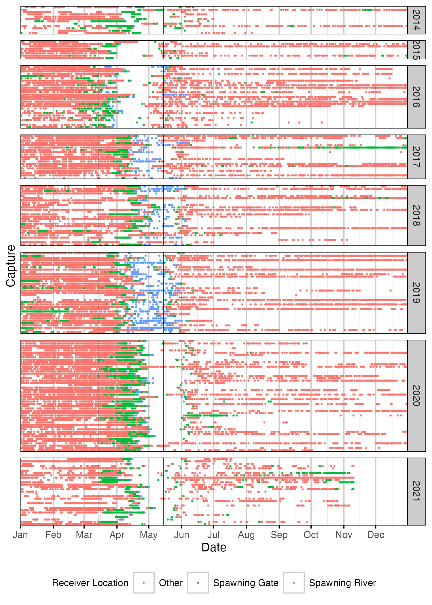
Figure 51. Date of detections of Rainbow Trout spawners by year. Colour indicates whether fish was detected in a spawning river, at a spawning gate or at a receiver not associated with a spawning area. Spawning period (March 15th to May 15th) is shown by solid black vertical lines. A fish was deemed to be spawning in a given year if it satisfied one of the following criteria: 1. Detected within a spawning river during the spawning period and a detection hiatus period of at least 7 days; 2. Detected within a spawning gate during the spawning period and a detection hiatus period of at least 21 days. Detections have been aggregated daily.
Condition
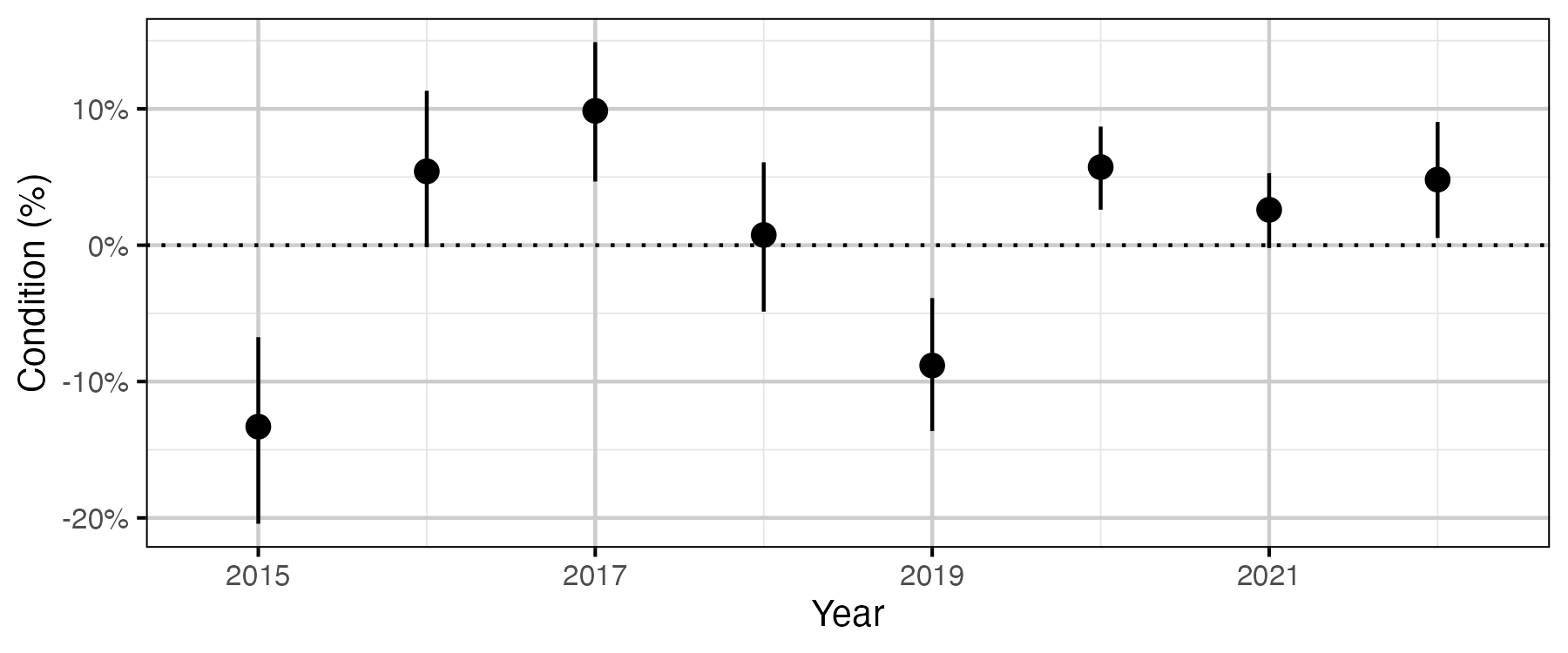
Figure 52. The percent change in body weight of a 700 mm Rainbow Trout spawner relative to an in-lake capture, by year (with 95% CRIs).
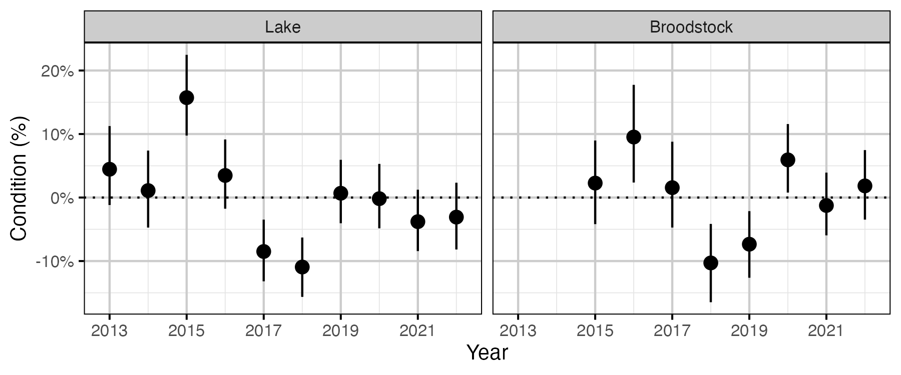
Figure 53. The percent change in the body weight of a 100 mm Rainbow Trout relative to a typical year, by year (with 95% CRIs).
Growth
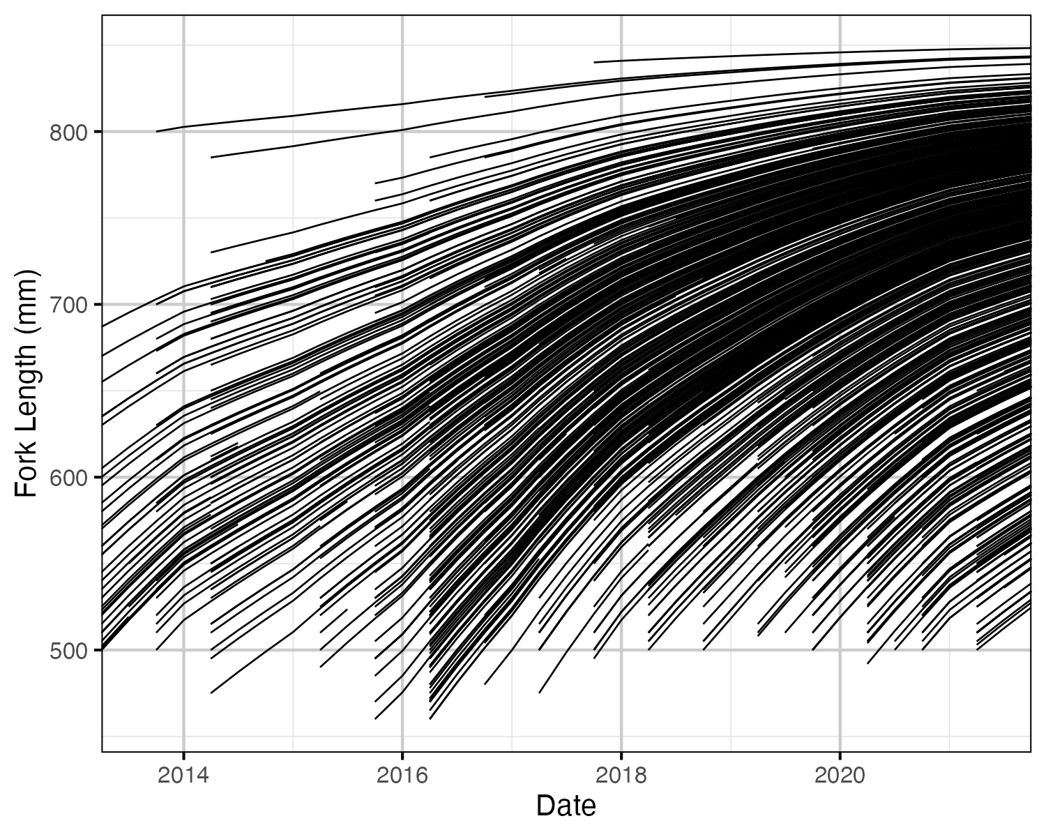
Figure 54. Estimated fork length for each fish by date.
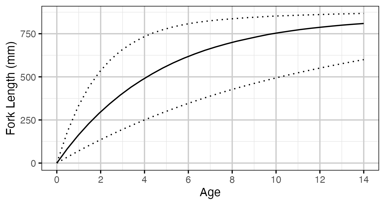
Figure 55. Estimated von Bertalanffy growth curve for a typical growth year.
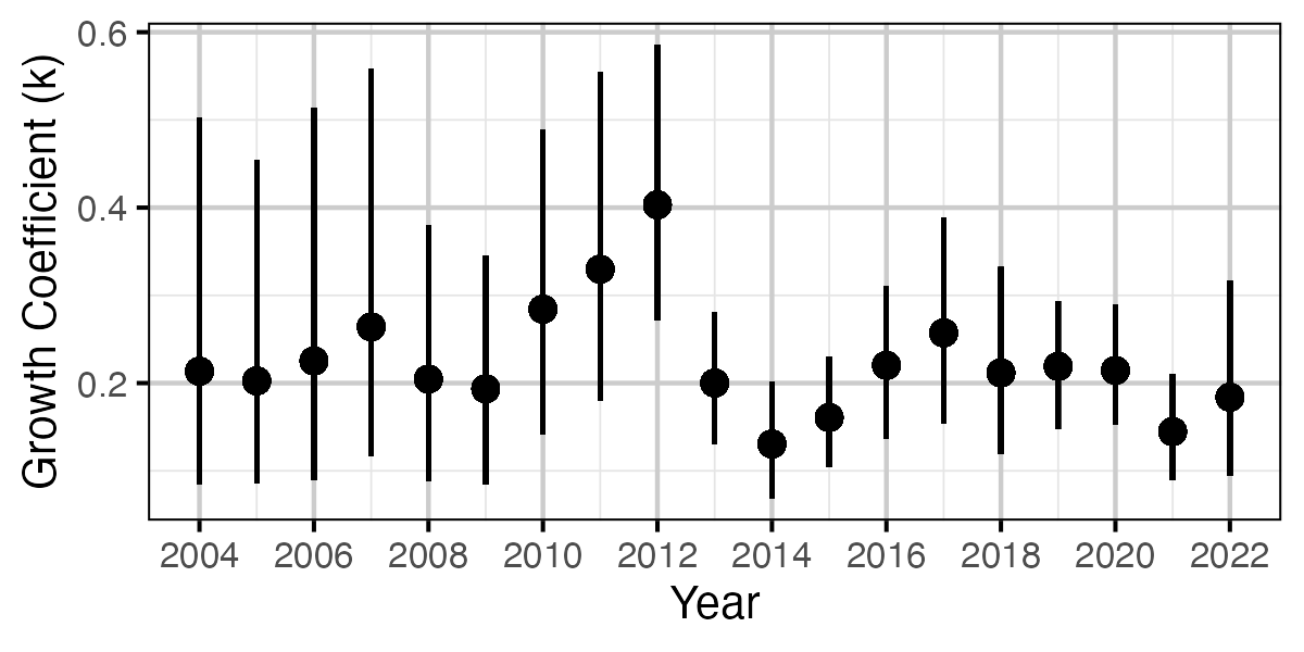
Figure 56. Estimated von Bertalanffy growth coefficient (k) by growth year (with 95% CIs).
Tag Loss
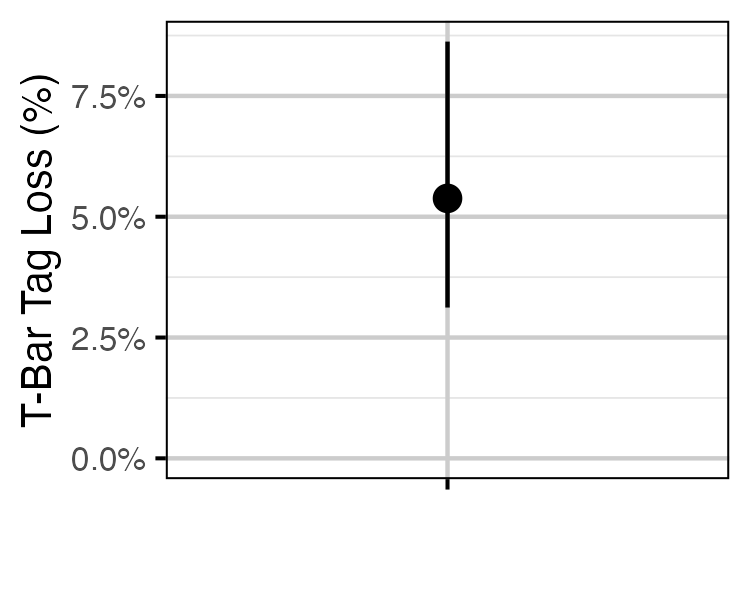
Figure 57. Estimated probability of the loss of a single T-bar tag (with 95% CIs).
Survival
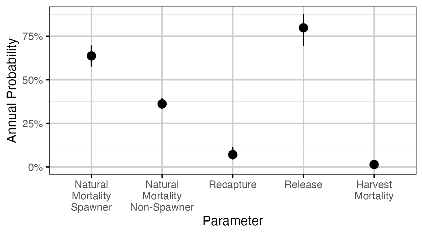
Figure 58. The estimated annual interval probabilities (with 95% CIs). Natural mortalities are for a medium sized fish (600-700 mm). Harvest mortality is the recapture probability multiplied by the probability of being harvested if recaptured, assuming that recapture can only occur once in a year. Release is the probability of being released if recaptured.
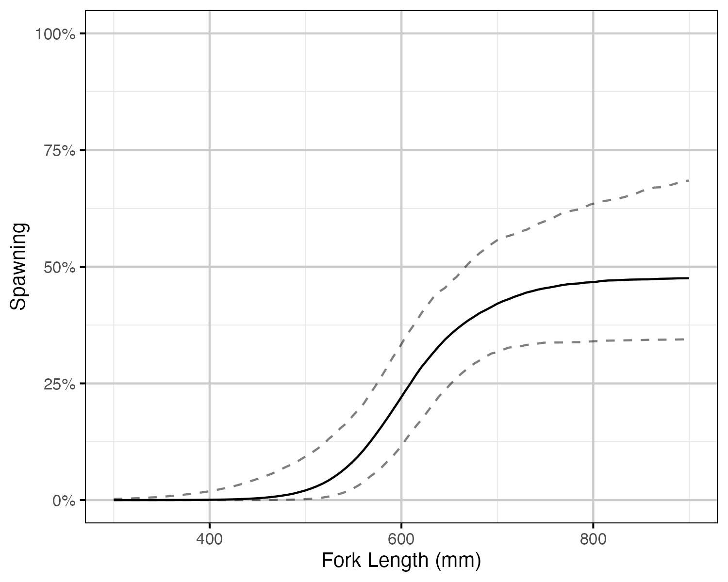
Figure 59. The probability of spawning by fork length (mm) for a typical year (with 95% CIs). Points represent whether a fish spawned at each spawning opportunity (i.e. spawning period and monitored).
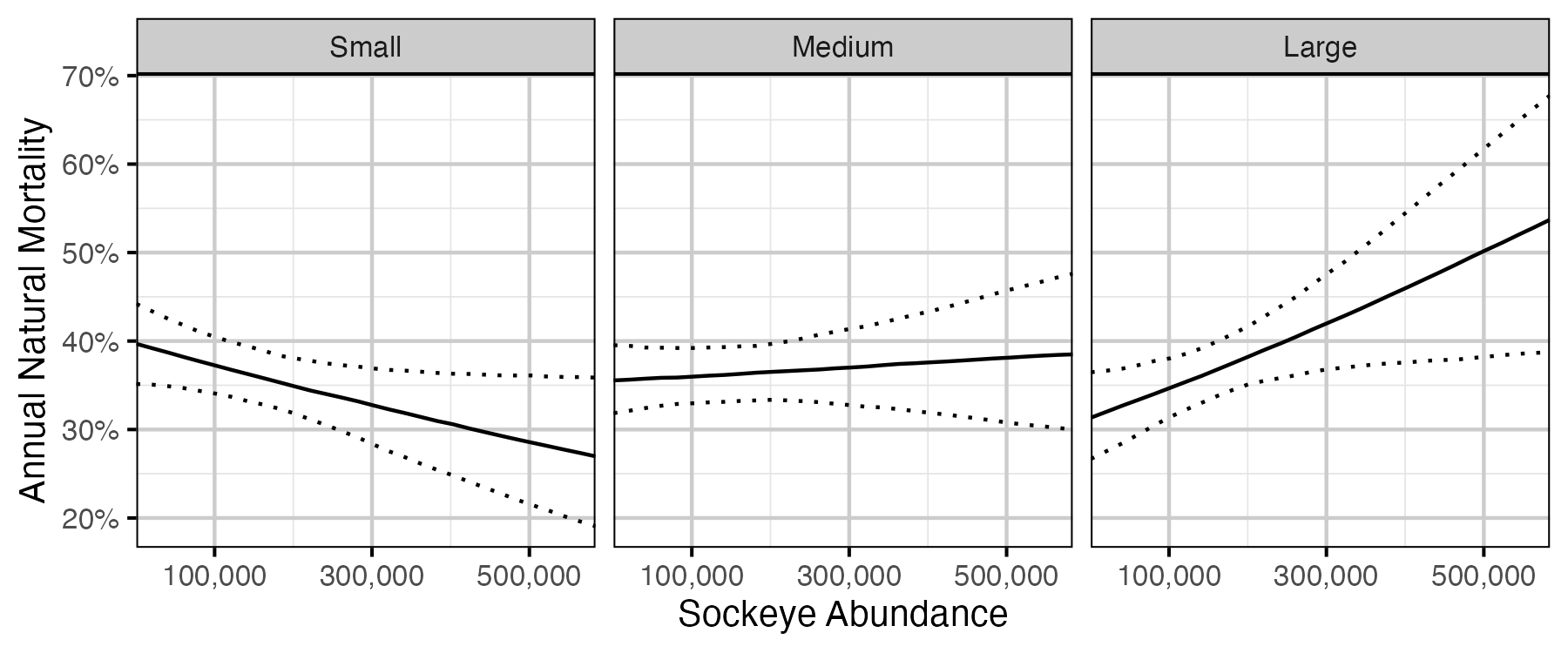
Figure 60. The estimated annual natural mortality by size class and sockeye abundance in the previous sockeye year (October 01 to September 30 the following year) (with 95% CIs).
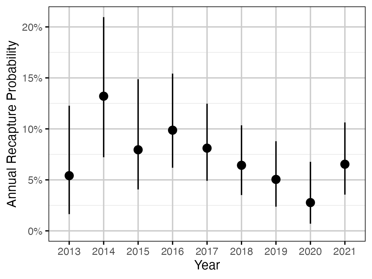
Figure 61. The estimated annual recapture probability by year (with 95% CIs).
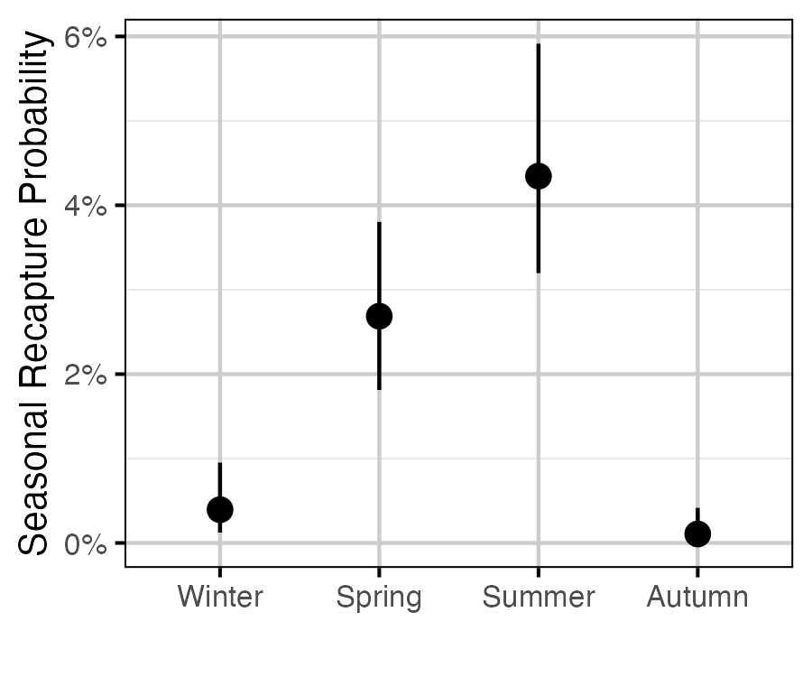
Figure 62. The estimated seasonal recapture probability for a typical year (with 95% CRIs).
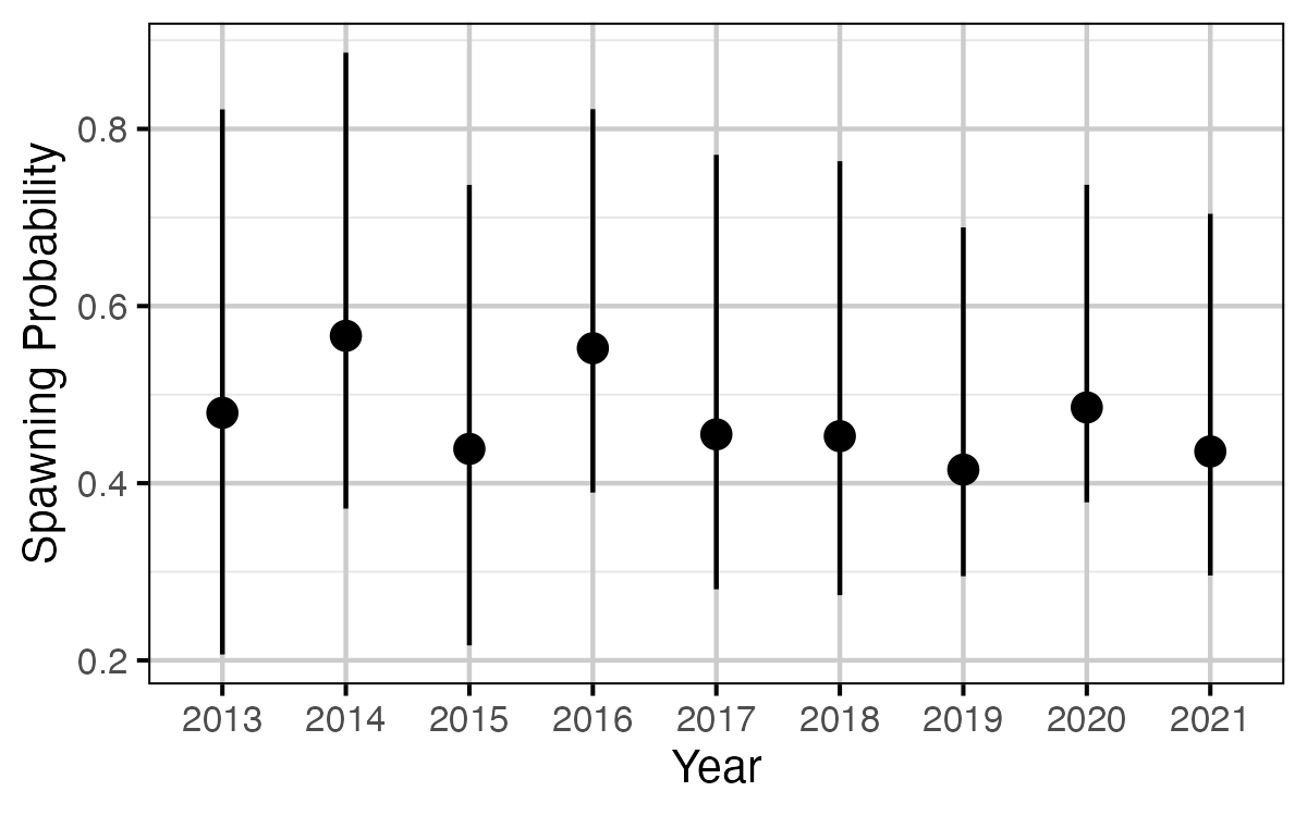
Figure 63. The estimated probability of a mature fish spawning, by year (with 95% CRIs).
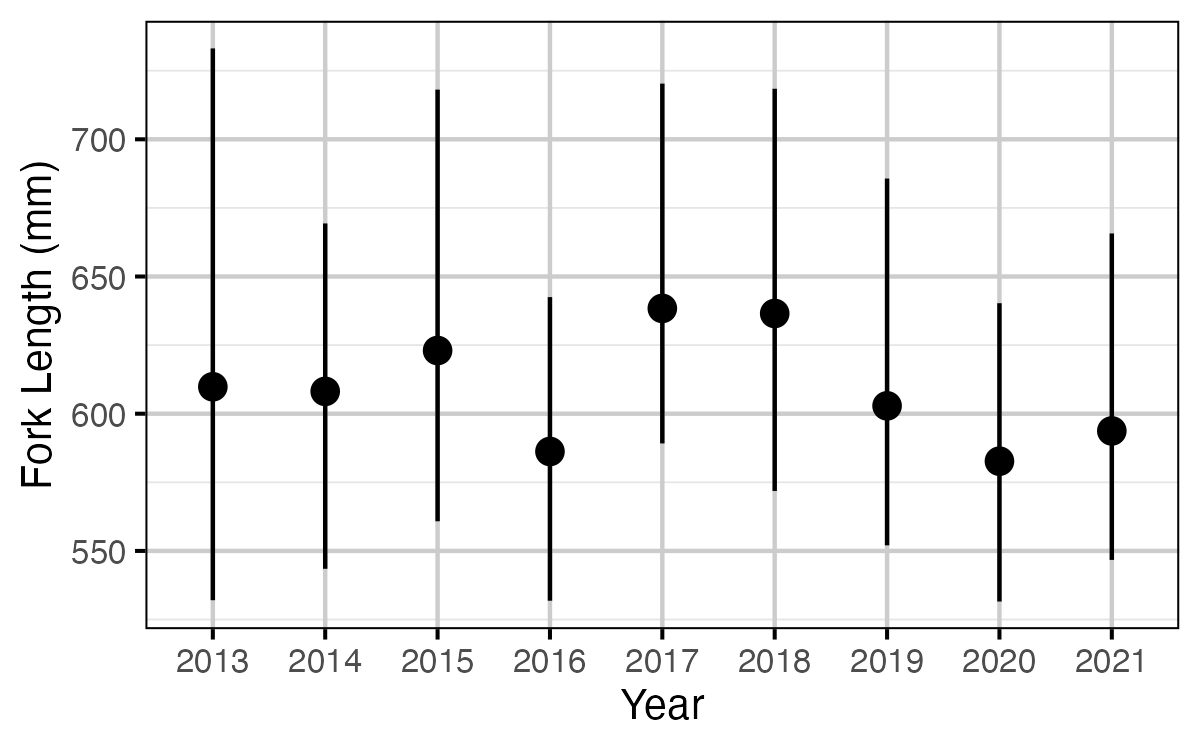
Figure 64. The estimated fork length (mm) at which 50% of fish are mature, by year (with 95% CRIs).
Mark-Recapture
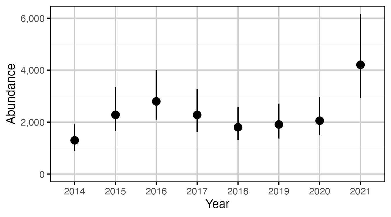
Figure 65. The estimated abundance of fish > 50 cm from in-lake captures and recaptures in 2014 to 2021, by year (with 95% CIs).
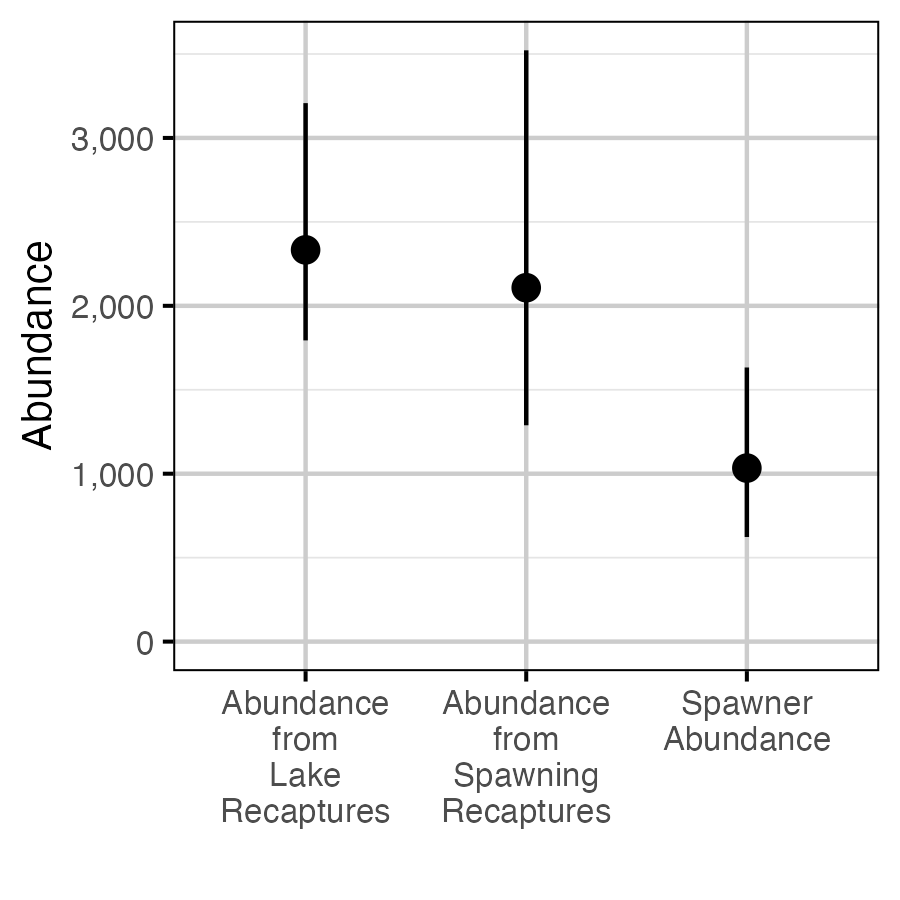
Figure 66. The estimated in-lake abundance of fish > 50 cm from in-lake recaptures and captures, averaged across years (2014-2021), in-lake abundance from spawner captures and recaptures averaged across years (2019-2021) and spawner abundance (with 95% CIs).
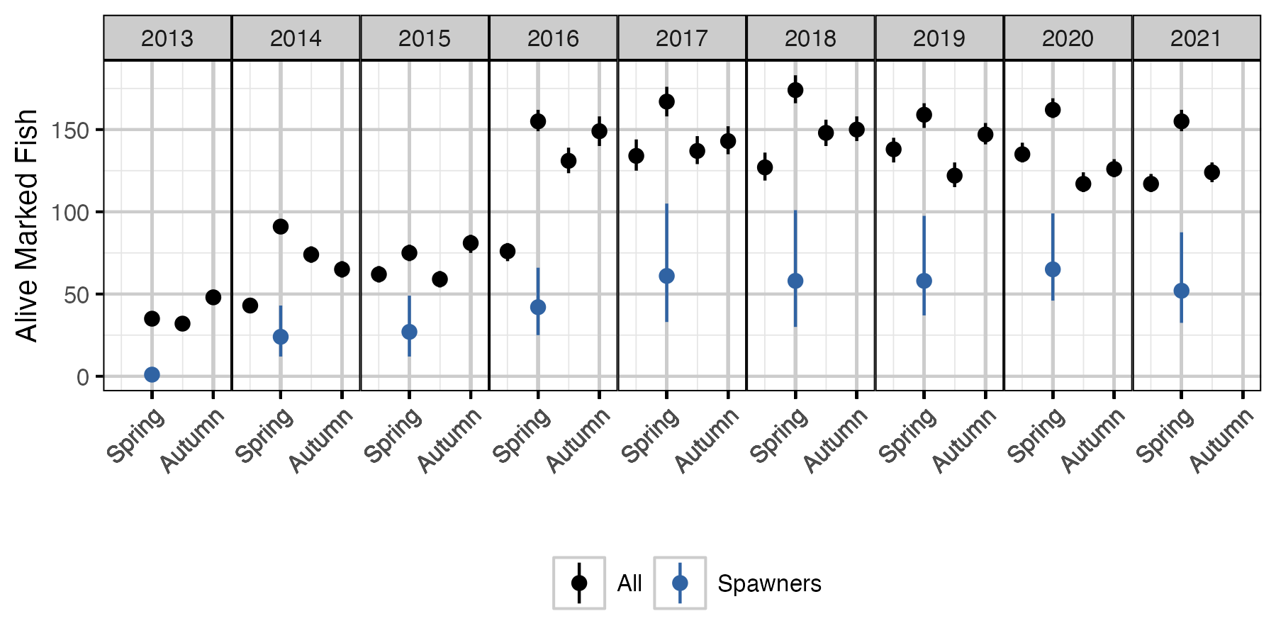
Figure 67. The estimated number of alive marked fish in the lake and marked spawning fish by seasonal time period (with 95% CIs). The number of marked spawners is based on the alive marked fish in the previous period.
Yield-per-Recruit
Slot Limit
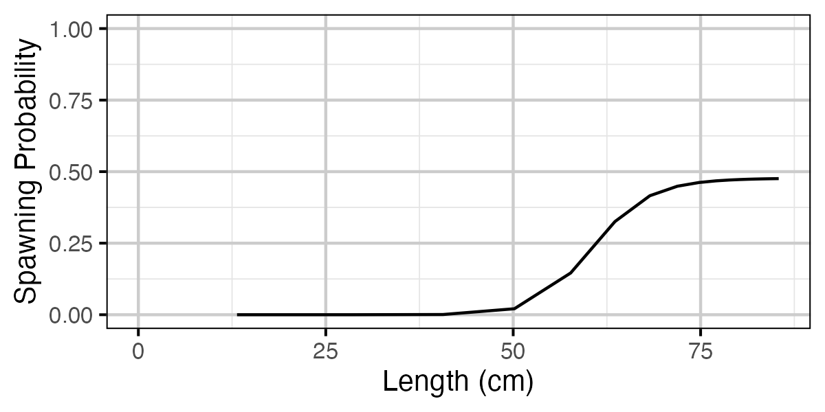
Figure 68. Calculated probability of spawning by length.
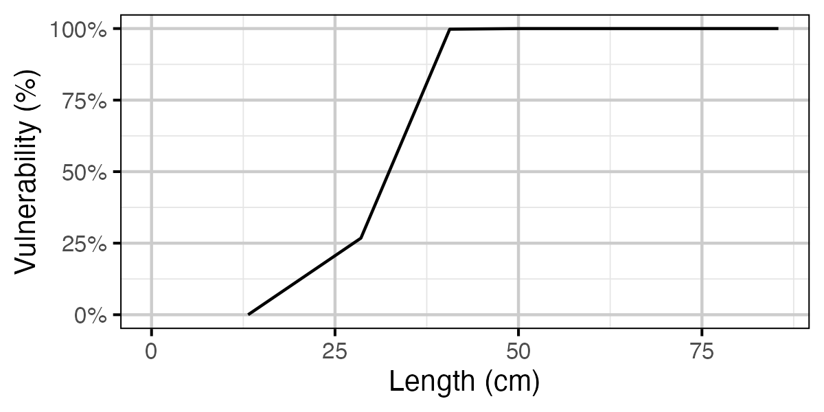
Figure 69. Calculated vulnerability to capture by length.
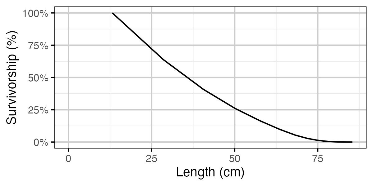
Figure 70. Calculated natural survivorship by length.
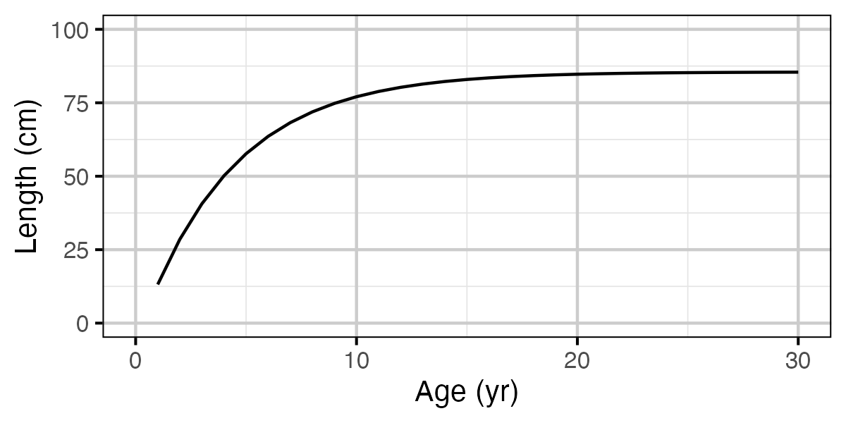
Figure 71. Calculated length by age.
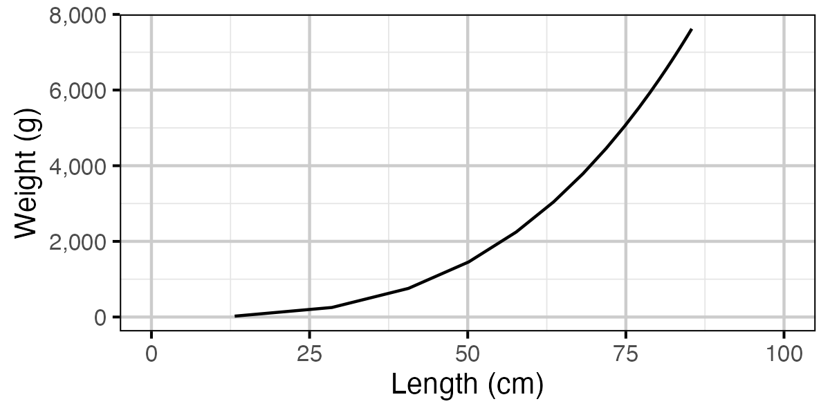
Figure 72. Calculated weight by length.
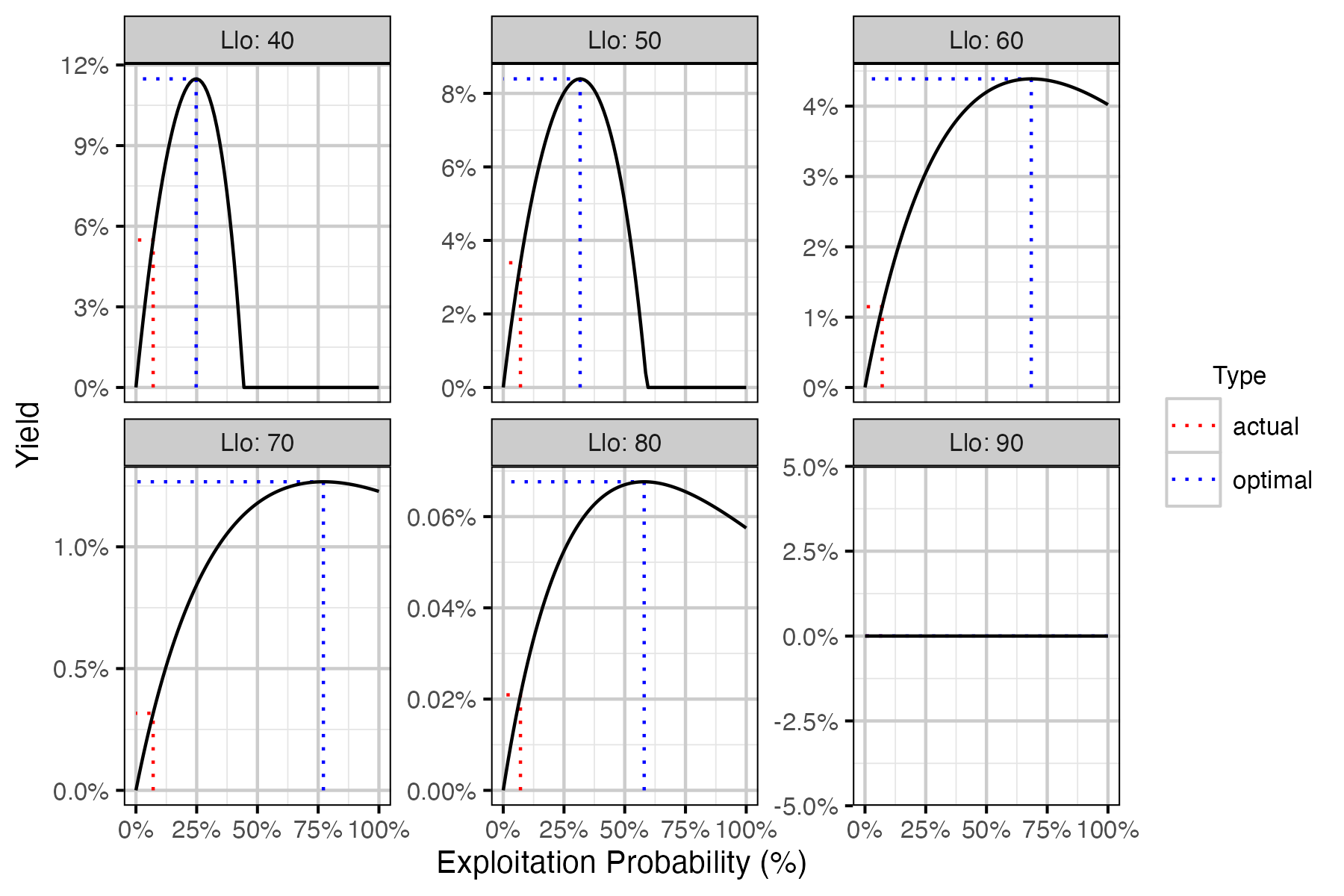
Figure 73. Calculated harvested number of fish as percent of the number of recruits at carrying capacity by annual interval exploitation rate, by Llo (lower slot limit).
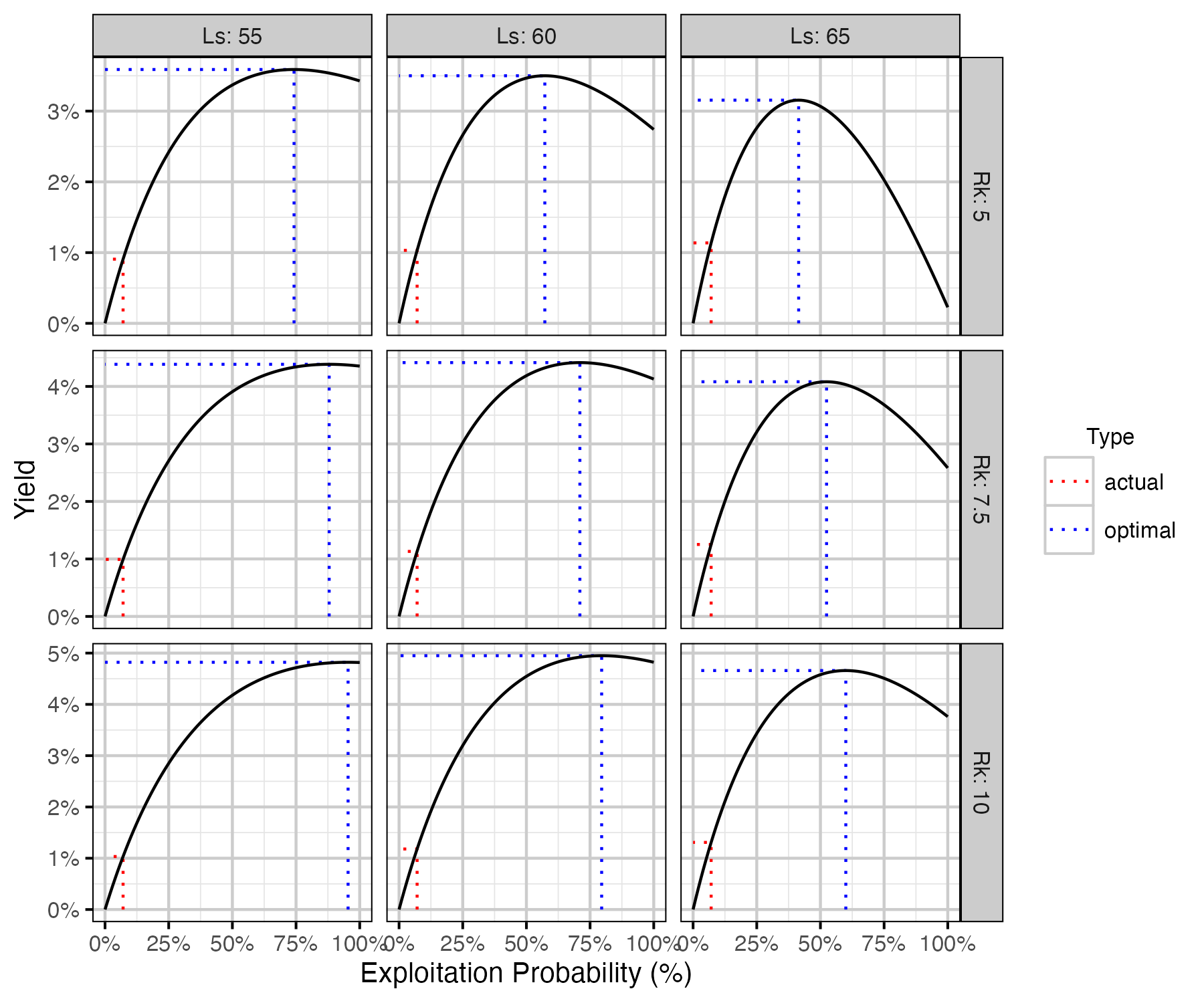
Figure 74. Calculated harvested number of fish as percent of the number of recruits at carrying capacity by annual interval exploitation rate, by Ls (length at 50% mature) and Rk (lifetime spawners per spawner at low density) with Llo (lower slot limit) held at 60 cm.
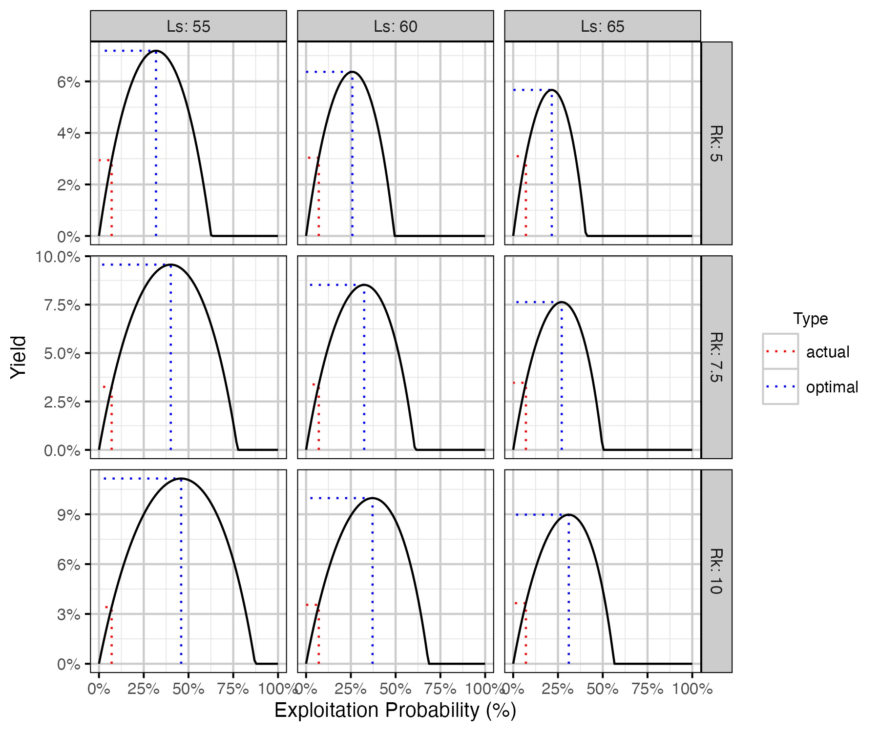
Figure 75. Calculated harvested number of fish as percent of the number of recruits at carrying capacity by annual interval exploitation rate, by Ls (length at 50% mature) and Rk (lifetime spawners per spawner at low density) with Llo (lower slot limit) held at 50 cm.
Acknowledgements
The organisations and individuals whose contributions have made this analysis report possible include:
- Quesnel Lake anglers for reporting their catches
- Habitat Conservation Trust Foundation (HCTF)
- and the anglers, hunters, trappers and guides who contribute to the Trust
- Ministry of Forests, Lands and Natural Resource Operations
- Lee Williston
- Mike Ramsay
- Greg Andrusak
- Reel Adventures
- Kerry Reed
- Vicky Lipinski