Quesnel Exploitation Analysis 2021
The suggested citation for this analytic appendix is:
Dalgarno, S. & Thorley, J.L. (2022) Quesnel Exploitation Analysis 2021. A Poisson Consulting Analytic Appendix. URL: https://www.poissonconsulting.ca/f/978976227.
Background
Quesnel Lake supports a recreational fishery for Rainbow Trout. To provide information on the natural and fishing mortality, Rainbow Trout were caught by angling and tagged with acoustic transmitters and/or a $100 and $10 reward tag.
Data Preparation
The outing, receiver deployment, detection, fish capture and recapture information were provided by the Ministry of Forests, Lands and Natural Resource Operations and added to a SQLite database.
The data were prepared for analysis using R version 4.2.1 (R Core Team 2021).
Receivers were assumed to have a detection range of 500 m. Detections were aggregated daily, where for each transmitter the receiver with the most number of detections was chosen. In the case of a tie, the receiver with the greatest coverage area was chosen. Only individuals with a fork length (FL) \(\geq\) 450 mm, an acoustic tag life \(\geq\) 365 days (if acoustically tagged) and a $100 and $10 reward tags were included in the survival analysis.
Statistical Analysis
Model parameters were estimated using Bayesian methods. The estimates were produced using JAGS (Plummer 2003) and STAN (Carpenter et al. 2017). For additional information on Bayesian estimation the reader is referred to McElreath (2016).
Unless stated otherwise, the Bayesian analyses used weakly informative normal and half-normal or uninformative beta prior distributions (Gelman, Simpson, and Betancourt 2017). The posterior distributions were estimated from 1500 Markov Chain Monte Carlo (MCMC) samples thinned from the second halves of 3 chains (Kery and Schaub 2011, 38–40). Model convergence was confirmed by ensuring that the potential scale reduction factor \(\hat{R} \leq 1.05\) (Kery and Schaub 2011, 40) and the effective sample size (Brooks et al. 2011) \(\textrm{ESS} \geq 150\) for each of the monitored parameters (Kery and Schaub 2011, 61).
The parameters are summarised in terms of the point estimate, lower and upper 95% credible limits (CLs) and the surprisal s-value (Greenland 2019). The estimate is the median (50th percentile) of the MCMC samples while the 95% CLs are the 2.5th and 97.5th percentiles. The s-value can be considered a test of directionality. More specifically it indicates how surprising (in bits) it would be to discover that the true value of the parameter is in the opposite direction to the estimate. An s-value of 4.3 bits, which is equivalent to a p-value (Kery and Schaub 2011; Greenland and Poole 2013) of 0.05, indicates that the surprise would be equivalent to throwing 4.3 heads in a row. The condition that non-essential explanatory variables have s-values \(\geq\) 4.3 bits provides a useful model selection heuristic (Kery and Schaub 2011).
The results are displayed graphically by plotting the modeled relationships between particular variables and the response(s) with the remaining variables held constant. In general, continuous and discrete fixed variables are held constant at their mean and first level values, respectively, while random variables are held constant at their typical values (expected values of the underlying hyperdistributions) (Kery and Schaub 2011, 77–82). When informative the influence of particular variables is expressed in terms of the effect size (i.e., percent or n-fold change in the response variable) with 95% credible intervals (CIs, Bradford, Korman, and Higgins 2005).
The analyses were implemented using R version 4.2.1
(R Core Team 2020) and the
mbr family of packages.
Model Descriptions
Condition
The expected weight of fish of a given length were estimated from the data using a mass-length model (He et al. 2008).
More specifically the model was based on the allometric relationship
\[ W = \alpha L^{\beta}\]
where \(W\) is the weight (mass), \(\alpha\) is the coefficent, \(\beta\) is the exponent and \(L\) is the length.
To improve chain mixing the relation was log-transformed, i.e.,
\[ \log(W) = \log(\alpha) + \beta \cdot \log(L)\]
Key assumptions of the condition model include:
- \(\alpha\) can vary randomly by year.
- The residual variation in weight is log-normally distributed.
Growth
The expected length of fish at a given age were estimated from broodstock data collected in the Horsefly River from 2015-2021 using a Von Bertalanffy growth curve model (von Bertalanffy 1938).
\[ L = L_\infty \cdot (1 - \exp(-k \cdot (A - t_0) ))\]
where \(A\) is the scale age in years and \(t_0\) is the extrapolated age at zero length.
Key assumptions of the growth model include:
- The residual variation in length is normally distributed.
Survival
The natural mortality and recapture probability were estimated using a Bayesian individual state-space survival model (Thorley and Andrusak 2017) with three month intervals. The survival model incorporated natural and handling mortality, acoustic detections, inter-section movement, T-bar tag loss, spawning, recapture and reporting.
T-bar tag loss was estimated from the number of tags reported from recaught double-tagged individuals (Fabrizio et al. 1999).
Fork length at spawning was calculated from the measured length at
capture (\(L_{i,fi}\)) plus the length increment expected under a Von
Bertalanffy Growth Curve (Walters & Martell, 2004)
\[L_{i,t} = L_{i,fi} + (L_{∞} − L_{i,fi} )(1 − e^{(−0.25 \cdot k(t −fi))})\]
where the 0.25 in the exponent adjusts for the fact that there are four
time periods per year. Parameters k and LInf were estimated from the
growth model.
A fish was considered to have spawned in a given year if one of the following conditions were met: detected within a spawning river during the spawning period with a detection hiatus of at least 7 days; or detected within a spawning gate during the spawning period with a detection hiatus of at least 14 days. Cutoff values for minimum hiatus periods were determined by inspecting the distribution of in-lake hiatus periods for fish detected in spawning rivers and the distribution of all hiatus periods for suspected spawners within the spawning period.
In addition to assumptions 1 to 2 and 4 to 10, in Thorley and Andrusak (2017), the model also assumes that:
- The effect of handling mortality is restricted to the first three month period after initial capture.
- The natural mortality varies by season, year and spawning.
- The spawning probability varies by year and fork length.
- The probability of tag loss is independent between tags on a fish.
- The probability of detection depends on whether a fish is alive or has died near or far from a receiver
- All recaptured fish have their tags removed.
- Reporting of recaptured fish with one or more T-bar tags is likely greater than 90%.
Yield-Per-Recruit
The optimal recapture rate (to maximize number of individuals caught) was calculated using a yield-per-recruit approach (Bison, O’Brien, and Martell 2003). Key assumptions include:
- The population is at equilibrium.
- All captured individuals < 500 mm are retained.
- All captured individuals \(\geq\) 500 mm are released.
- Handling mortality is 10%.
- The life-history parameters are fixed.
- There are no Allee effects.
- There are no limitations on prey species.
The optimal yield was also calculated with no slot limit.
Model Templates
Growth
.model {
  bLInf ~ dnorm(900, 200^-2) T(0, )
  bK ~ dnorm(0.2, 1^-2) T(0, )
  bT0 ~ dnorm(0, 2^-1)

  sLength ~ dnorm(0, 100^-2) T(0, )
  for (i in 1:length(Length)) {
    eLength[i] <- bLInf * (1 - exp(-bK * (Age[i] - bT0)))
    Length[i] ~ dnorm(eLength[i], sLength^-2) T(0, )
  }
Block 1. Growth model description.
Condition
  data {
    int nannual;
    int nObs;

    vector[nObs] length;
    vector[nObs] weight;
    int annual[nObs];
  }

  parameters {
    real bWeight;
    real bLength;
    real<lower=0> sWeightAnnual;

    vector[nannual] bWeightAnnual;
    real<lower=0> sWeight;
  }

  model {

    vector[nObs] eWeight;

    bWeight ~ normal(-11, 2);
    bLength ~ normal(3, 1);

    sWeightAnnual ~ normal(0, 1);

    for (i in 1:nannual) {
        bWeightAnnual[i] ~ normal(0, sWeightAnnual);
    }

    sWeight ~ normal(0, 1);
    for(i in 1:nObs) {
      eWeight[i] = exp(bWeight + bLength * log(length[i]) + bWeightAnnual[annual[i]]);
      weight[i] ~ lognormal(log(eWeight[i]), sWeight);
    }
  }
Block 2. Condition model description.
Survival
.model{
  bMortality ~ dnorm(-3, 3^-2)
  bMortalitySpawning ~ dnorm(0, 2^-2)
  bSpawning ~ dnorm(0, 2^-2)
  bSpawningLength ~ dnorm(0, 2^-2)
  bTagLoss ~ dbeta(101, 1001)

  bDetectedAlive ~ dbeta(1, 1)
  bDieNear ~ dbeta(1, 1)
  bDetectedDeadNear ~ dbeta(10, 1)
  bDetectedDeadFar ~ dbeta(1, 10)
  bMoved ~ dbeta(1, 1)
  bRecaptured ~ dbeta(1, 1)
  bReported ~ dbeta(10, 1)
  sSpawningAnnual ~ dexp(1)
  for (i in 1:nAnnual) {
    bSpawningAnnual[i] ~ dnorm(0, sSpawningAnnual^-2)
  }
  bMortalitySeason[1] <- 0
  for (i in 2:nSeason) {
    bMortalitySeason[i] ~ dnorm(0, 2^-2)
  }
  sMortalityAnnual ~ dexp(1)
  for (i in 1:nAnnual) {
    bMortalityAnnual[i] ~ dnorm(0, sMortalityAnnual^-2)
  }

  for (i in 1:nCapture){
    eDetectedAlive[i] <- bDetectedAlive
    eDieNear[i] ~ dbern(bDieNear)
    eDetectedDeadNear[i] <- bDetectedDeadNear
    eDetectedDeadFar[i] <- bDetectedDeadFar
    eDetectedDead[i] <- eDieNear[i] * eDetectedDeadNear[i] + (1 - eDieNear[i]) * eDetectedDeadFar[i]

    logit(eMortality[i,PeriodCapture[i]]) <- bMortality + bMortalitySeason[Season[i,PeriodCapture[i]]] + bMortalityAnnual[Annual[i,PeriodCapture[i]]]

    eTagLoss[i,PeriodCapture[i]] <- bTagLoss
    eMoved[i,PeriodCapture[i]] <- bMoved
    eRecaptured[i,PeriodCapture[i]] <- bRecaptured
    eReported[i,PeriodCapture[i]] <- bReported

    InLake[i,PeriodCapture[i]] <- 1
    Alive[i,PeriodCapture[i]] ~ dbern(1-eMortality[i,PeriodCapture[i]])
    TBarTag100[i,PeriodCapture[i]] ~ dbern(1-eTagLoss[i,PeriodCapture[i]])
    TBarTag10[i,PeriodCapture[i]] ~ dbern(1-eTagLoss[i,PeriodCapture[i]])

    eDetected[i,PeriodCapture[i]] <- Alive[i,PeriodCapture[i]] * eDetectedAlive[i] + (1-Alive[i,PeriodCapture[i]]) * eDetectedDead[i]
    Detected[i,PeriodCapture[i]] ~ dbern(Monitored[i,PeriodCapture[i]] * eDetected[i,PeriodCapture[i]])
    Moved[i,PeriodCapture[i]] ~ dbern(Alive[i,PeriodCapture[i]] * Detected[i,PeriodCapture[i]] * eMoved[i,PeriodCapture[i]])

    Recaptured[i,PeriodCapture[i]] ~ dbern(Alive[i,PeriodCapture[i]] * eRecaptured[i,PeriodCapture[i]])
    Reported[i,PeriodCapture[i]] ~ dbern(Recaptured[i,PeriodCapture[i]] * eReported[i,PeriodCapture[i]] * step(TBarTag100[i,PeriodCapture[i]] + TBarTag10[i,PeriodCapture[i]] - 1))

  for(j in (PeriodCapture[i]+1):nPeriod) {
    logit(eSpawning[i,j]) <- bSpawning + bSpawningLength * Length[i,j] + bSpawningAnnual[Annual[i,j]]
    Spawned[i,j] ~ dbern(Alive[i,j-1] * Monitored[i,j] * SpawningPeriod[i,j] * eSpawning[i,j])

    logit(eMortality[i,j]) <- bMortality + bMortalitySpawning * Spawned[i,j] + bMortalitySeason[Season[i,j]] + bMortalityAnnual[Annual[i,j]]
    eDetected[i,j] <- Alive[i,j] * eDetectedAlive[i] + (1-Alive[i,j]) * eDetectedDead[i]

    eTagLoss[i,j] <- bTagLoss
    eMoved[i,j] <- bMoved
    eRecaptured[i,j] <- bRecaptured
    eReported[i,j] <- bReported

    InLake[i,j] ~ dbern(InLake[i,j-1] * (1 - Recaptured[i,j-1]))
    Alive[i,j] ~ dbern(Alive[i,j-1] * (1 - Recaptured[i,j-1]) * (1-eMortality[i,j]))
    TBarTag100[i,j] ~ dbern(TBarTag100[i,j-1] * (1-Recaptured[i,j-1]) * (1-eTagLoss[i,j]))
    TBarTag10[i,j] ~ dbern(TBarTag10[i,j-1] * (1-Recaptured[i,j-1]) * (1-eTagLoss[i,j]))

    Detected[i,j] ~ dbern(InLake[i,j] * Monitored[i,j] * eDetected[i,j])
    Moved[i,j] ~ dbern(Alive[i,j] * Detected[i,j] * eMoved[i,j])

    Recaptured[i,j] ~ dbern(Alive[i,j] * eRecaptured[i,j])
    Reported[i,j] ~ dbern(Recaptured[i,j] * eReported[i,j] * step(TBarTag100[i,j] + TBarTag10[i,j] - 1))
  }
  }
Block 3. Survival model description.
Results
Tables
Growth
Table 1. Model coefficients.
| term | estimate | sd | zscore | lower | upper | pvalue |
|---|---|---|---|---|---|---|
| bK | 0.2295451 | 0.0680279 | 3.4539894 | 0.1230586 | 0.3897374 | 0.0006662 |
| bLInf | 889.4638952 | 72.6192558 | 12.4511860 | 798.2282422 | 1078.9269369 | 0.0006662 |
| bT0 | 0.3421945 | 0.8634450 | 0.3097905 | -1.5199278 | 1.7933157 | 0.7161892 |
| sLength | 57.4970288 | 3.1067395 | 18.5711849 | 51.9442684 | 64.1285862 | 0.0006662 |
Table 2. Model summary.
| n | K | nchains | niters | nthin | ess | rhat | converged |
|---|---|---|---|---|---|---|---|
| 179 | 4 | 3 | 500 | 100 | 153 | 1.014 | TRUE |
Condition
Table 3. Parameter descriptions.
| Parameter | Description |
|---|---|
annual[i] |
Year ith fish was captured as a factor |
bWeight |
Intercept of log(eWeight) |
bWeightAnnual[i] |
Effect of ith annual on bWeight |
bWeightLength |
Intercept of effect of log(length) on bWeight |
eWeight[i] |
Expected weight of ith fish |
length[i] |
Fork length of ith fish |
sWeight |
Log standard deviation of residual variation in
log(Weight) |
sWeightAnnual |
Log standard deviation of bWeightAnnual |
weight[i] |
Recorded weight of ith fish |
Table 4. Model coefficients.
| term | estimate | sd | zscore | lower | upper | pvalue |
|---|---|---|---|---|---|---|
| bLength | 2.9987995 | 0.0316225 | 94.846043 | 2.9380074 | 3.0625907 | 0.0006662 |
| bWeight | -11.3498512 | 0.2042258 | -55.579201 | -11.7654447 | -10.9474587 | 0.0006662 |
| sWeight | 0.1431402 | 0.0030844 | 46.449721 | 0.1375974 | 0.1497259 | 0.0006662 |
| sWeightAnnual | 0.0768943 | 0.0271453 | 3.028439 | 0.0456621 | 0.1515867 | 0.0006662 |
Table 5. Model summary.
| n | K | nchains | niters | nthin | ess | rhat | converged |
|---|---|---|---|---|---|---|---|
| 1056 | 4 | 3 | 500 | 10 | 1138 | 1.002 | TRUE |
Survival
Table 6. Parameter descriptions.
| Parameter | Description |
|---|---|
bDetectedAlive |
Seasonal probability of detection if in-lake |
bDetectedDeadFar |
Seasonal probability of detection if in-lake and dead far from a receiver |
bDetectedDeadNear |
Seasonal probability of detection if in-lake and dead near a receiver |
bDieNear |
Lifetime probability of dying near versus far from a receiver |
bMortality |
Log odds seasonal probability of dying of natural causes |
bMortalityAnnual |
Effect of ith Year on bMortality |
bMortalitySeason |
Effect of ith Season on bMortality |
bMortalitySpawning |
Effect of spawning on bMortality |
bMoved |
Seasonal probability of being detected moving between sections if alive |
bRecaptured |
Seasonal probability of being recaptured if alive |
bRelease |
Probability of being released if recaptured and untagged |
bReported |
Probability of being reported if recaptured with one or more T-bar tags |
bSpawning |
Seasonal probability of spawning if in spawning period. |
bSpawningAnnual |
Effect of ith Year on bSpawning |
bSpawningLength |
Effect of Fork Length on bSpawning |
bTagLoss |
Seasonal probability of loss for a single T-bar tag |
sMortalityAnnual |
Standard deviation of residual variation in
bMortalityAnnual |
sSpawningAnnual |
Standard deviation of residual variation in
bSpawningAnnual |
Table 7. Model coefficients.
| term | estimate | sd | zscore | lower | upper | pvalue |
|---|---|---|---|---|---|---|
| bDetectedAlive | 0.9641062 | 0.0036303 | 265.561897 | 0.9565662 | 0.9706165 | 0.0006662 |
| bDetectedDeadFar | 0.0165180 | 0.0032184 | 5.156941 | 0.0106466 | 0.0234644 | 0.0006662 |
| bDetectedDeadNear | 0.6977680 | 0.0234935 | 29.660188 | 0.6496680 | 0.7399145 | 0.0006662 |
| bDieNear | 0.1765838 | 0.0209512 | 8.450340 | 0.1385571 | 0.2192742 | 0.0006662 |
| bMortality | -2.5037877 | 0.1926015 | -13.067100 | -2.9048225 | -2.1638165 | 0.0006662 |
| bMortalitySeason[2] | -0.5052270 | 0.2441138 | -2.048420 | -0.9700982 | -0.0201799 | 0.0433045 |
| bMortalitySeason[3] | 0.7992381 | 0.1910335 | 4.227951 | 0.4460471 | 1.1990131 | 0.0006662 |
| bMortalitySeason[4] | 0.5781563 | 0.2005353 | 2.892682 | 0.1986316 | 0.9752009 | 0.0033311 |
| bMortalitySpawning | 1.7795906 | 0.1958139 | 9.062977 | 1.3805817 | 2.1626955 | 0.0006662 |
| bMoved | 0.8262282 | 0.0078011 | 105.874826 | 0.8101659 | 0.8406585 | 0.0006662 |
| bRecaptured | 0.0211410 | 0.0023934 | 8.893420 | 0.0169482 | 0.0261738 | 0.0006662 |
| bReported | 0.9920432 | 0.0115708 | 85.423615 | 0.9576959 | 0.9997300 | 0.0006662 |
| bSpawning | -0.7754943 | 0.1901161 | -4.094442 | -1.1568083 | -0.4123476 | 0.0019987 |
| bSpawningLength | 1.3364276 | 0.1406634 | 9.521426 | 1.0776886 | 1.6304789 | 0.0006662 |
| bTagLoss | 0.0575715 | 0.0057642 | 10.043427 | 0.0471327 | 0.0695807 | 0.0006662 |
| sMortalityAnnual | 0.2117021 | 0.1465518 | 1.627167 | 0.0294504 | 0.5948119 | 0.0006662 |
| sSpawningAnnual | 0.3393802 | 0.2160980 | 1.713510 | 0.0483291 | 0.9083506 | 0.0006662 |
Table 8. Model summary.
| n | K | nchains | niters | nthin | ess | rhat | converged |
|---|---|---|---|---|---|---|---|
| 23870 | 17 | 3 | 500 | 100 | 106 | 1.044 | FALSE |
Yield-per-Recruit
Slot Limit
Table 9. Rainbow Trout yield-per-recruit calculations including the capture probability (pi), exploitation rate (u), and average age, length and weight of fish harvested.
| Type | pi | u | Yield | Age | Length | Weight | Effort |
|---|---|---|---|---|---|---|---|
| actual | 0.0819200 | 0.0819200 | 0.0882968 | 4.135190 | 49.00099 | 1435.637 | 0.8112219 |
| optimal | 0.5354855 | 0.5354855 | 0.3191909 | 3.593554 | 44.55992 | 1095.597 | 7.2775134 |
Table 10. Rainbow Trout yield-per-recruit model parameters.
| Parameter | Value | Description | Source |
|---|---|---|---|
| tmax | 30.000 | The maximum age (yr). | Professional Judgement |
| k | 0.230 | The VB growth coefficient (yr-1). | Current Study |
| Linf | 88.946 | The VB mean maximum length (cm). | Current Study |
| t0 | 0.342 | The (theoretical) age at zero length (yr). | Current Study |
| k2 | 0.150 | The VB growth coefficient after length L2 (yr-1). | Default |
| Linf2 | 100.000 | The VB mean maximum length after length L2 (cm). | Default |
| L2 | 1000.000 | The length (or age if negative) at which growth switches from the | |
| first to second phase (cm or yr). | Default | ||
| Wb | 3.000 | The weight (as a function of length) scaling exponent. | Default |
| Ls | 65.000 | The length (or age if negative) at which 50 % mature (cm or yr). | Professional Judgement |
| Sp | 100.000 | The maturity (as a function of length) power. | Default |
| es | 0.500 | The annual probability of a mature fish spawning. | Professional Judgement |
| Sm | 0.428 | The spawning mortality probability. | Current Study |
| fb | 1.000 | The fecundity (as a function of weight) scaling exponent. | Default |
| tR | 1.000 | The age from which survival is density-independent (yr). | Default |
| BH | 1.000 | Recruitment follows a Beverton-Holt (1) or Ricker (0) relationship. | Default |
| Rk | 12.500 | The lifetime spawners per spawner at low density (or the egg to tR survival if between 0 and 1). | (thorley_duncan_2018?) |
| n | 0.351 | The annual interval natural mortality rate from age tR. | Current Study |
| nL | 0.200 | The annual interval natural mortality rate from length Ln. | Default |
| Ln | 1000.000 | The length (or age if negative) at which the natural mortality | |
| rate switches from n to nL (cm or yr). | Constant Mortality | ||
| Lv | 30.000 | The length (or age if negative) at which 50 % vulnerable to harvest | |
| (cm or yr). | Professional Judgement | ||
| Vp | 20.000 | The vulnerability to harvest (as a function of length) power. | Professional Judgement |
| Llo | 0.000 | The lower harvest slot length (cm). | Default |
| Lup | 50.000 | The upper harvest slot length (cm). | Fishery Regulation |
| Nc | 0.000 | The slot limits non-compliance probability. | Default |
| pi | 0.082 | The annual capture probability. | Current Study |
| rho | 0.000 | The release probability. | Default |
| Hm | 0.100 | The hooking mortality probability. | Professional Judgement |
| Rmax | 1.000 | The number of recruits at the carrying capacity (ind). | Default |
| Wa | 0.010 | The (extrapolated) weight of a 1 cm individual (g). | Default |
| fa | 1.000 | The (theoretical) fecundity of a 1 g female (eggs). | Default |
| q | 0.100 | The catchability (annual probability of capture) for a unit of | |
| effort. | Default | ||
| RPR | 1.000 | The relative proportion of recruits that are of the ecotype. | Default |
Figures
Captures
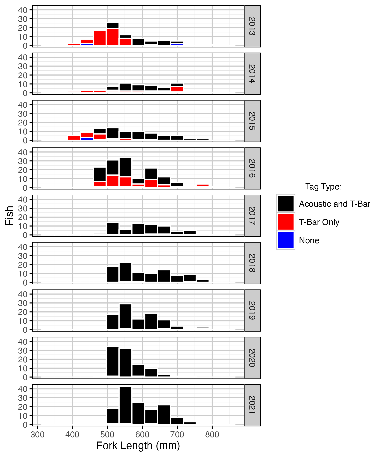
Figure 1. Rainbow Trout captures by fork length, year, and tag type.
Sections
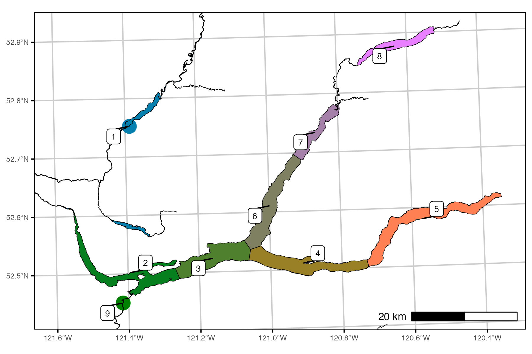
Figure 2. Quesnel Lake sections. Color code is used to identify sections throughout analysis.
Coverage
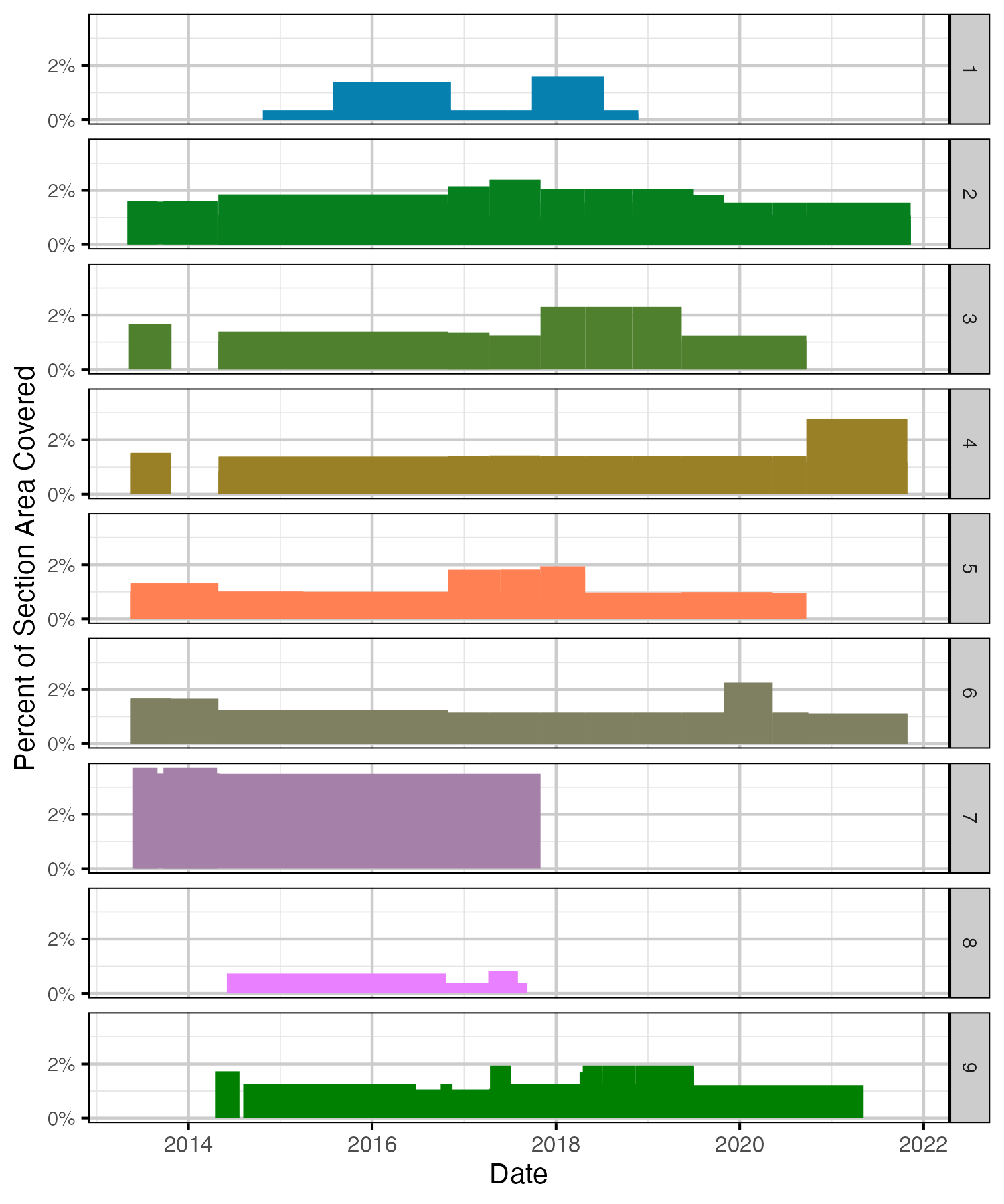
Figure 3. Receiver coverage of section area by date.
Detections
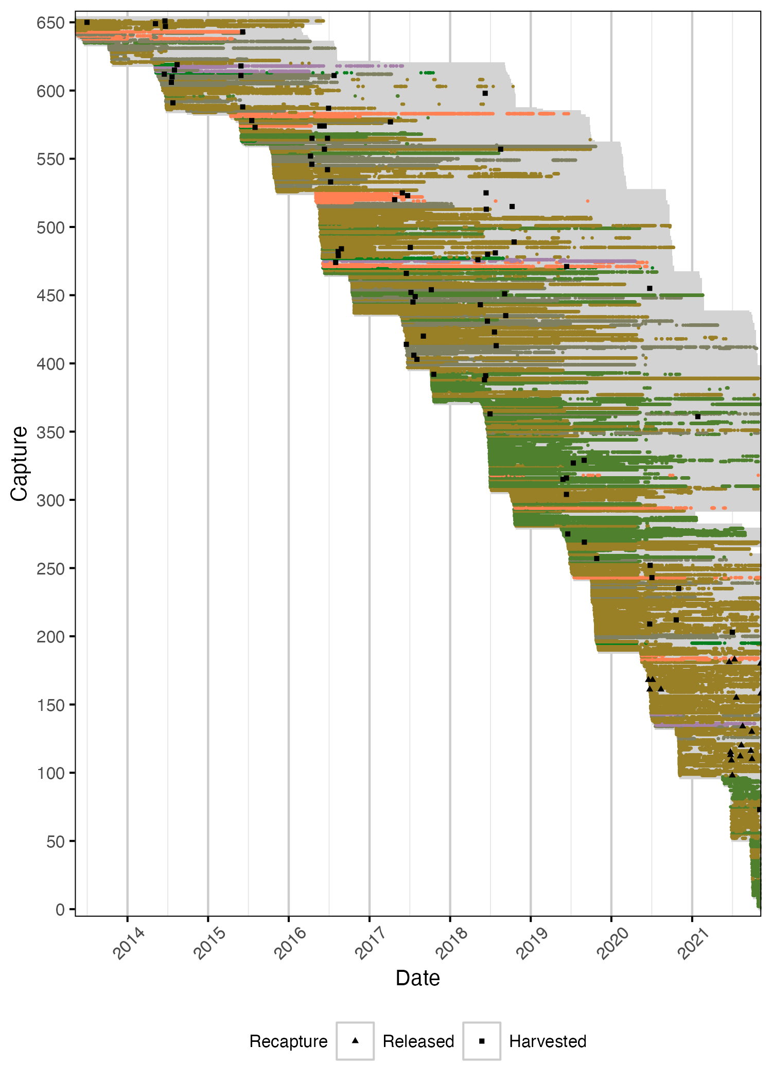
Figure 4. Date of detections for each acoustically tagged Rainbow Trout. Grey segments indicate estimated tag life from capture date. Detections have been aggregated daily.
Spawners
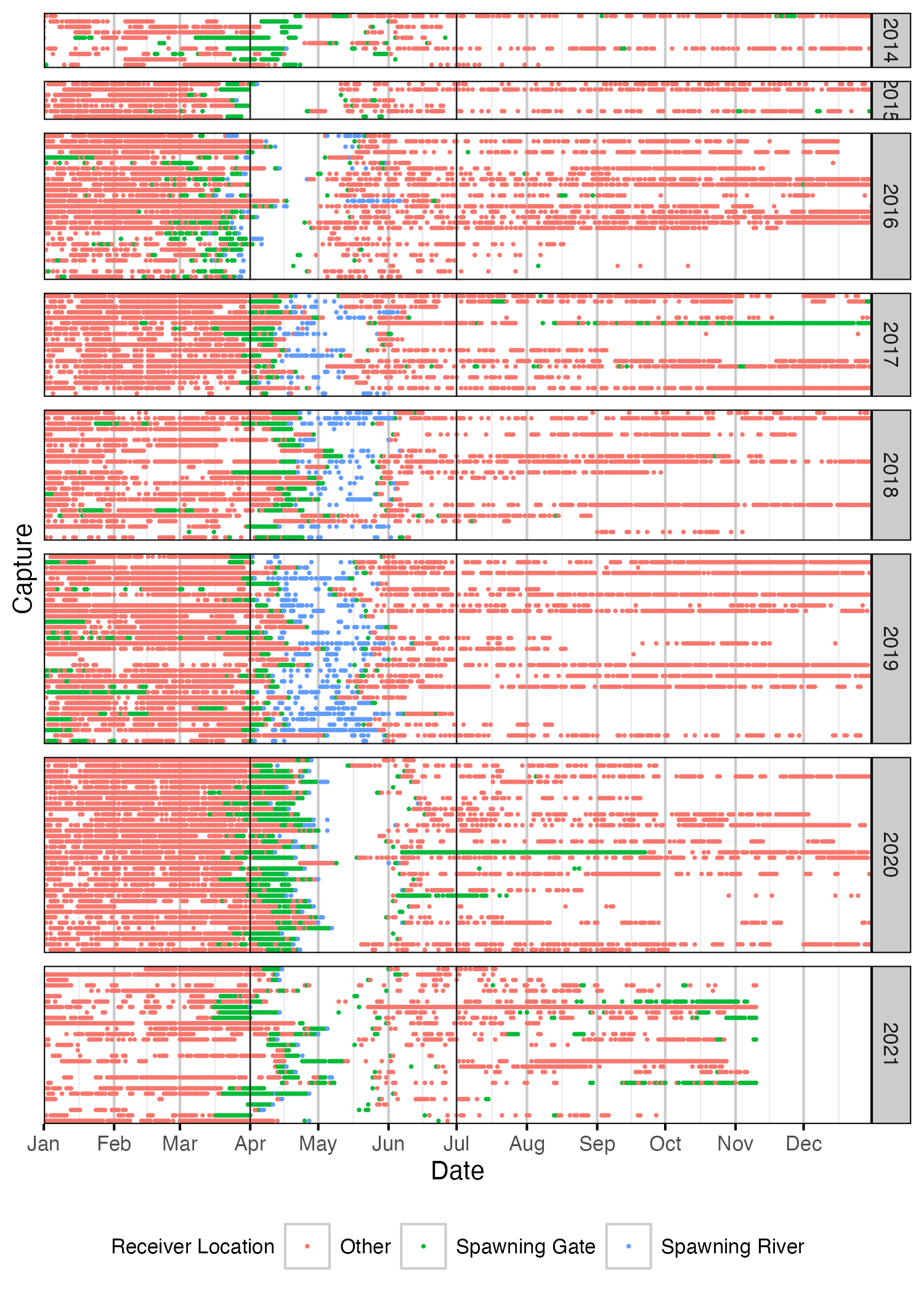
Figure 5. Date of detections of Rainbow Trout spawners by year. Colour indicates whether fish was detected in a spawning river, at a spawning gate or at a receiver not associated with a spawning area. Spawning period (March 15th to May 15th) is shown by solid black vertical lines. A fish was deemed to be spawning in a given year if it satisfied one of the following criteria: 1. Detected within a spawning river during the spawning period and a detection hiatus period of at least 7 days; 2. Detected within a spawning gate during the spawning period and a detection hiatus period of at least 14 days. Detections have been aggregated daily.
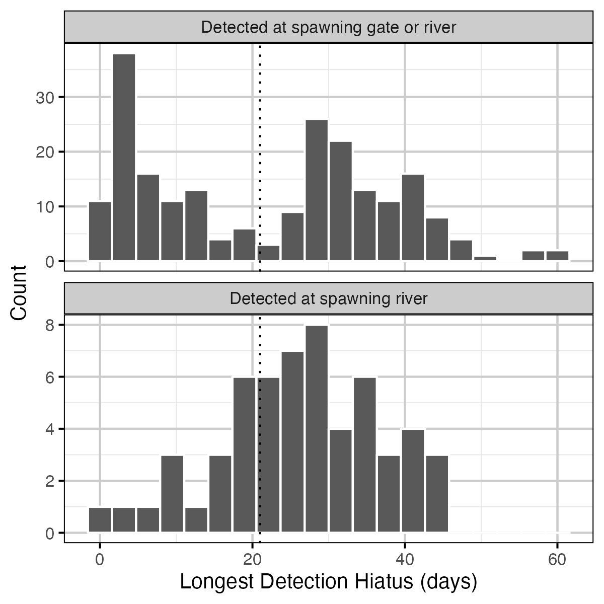
Figure 6. Longest detection hiatus during the spawning window (April to June) for potential spawners. Spawning gates are receivers at or near the mouth of a spawning river. Spawning rivers include Horsefly River and Mitchell River. Dotted vertical line is 21 days.
Growth
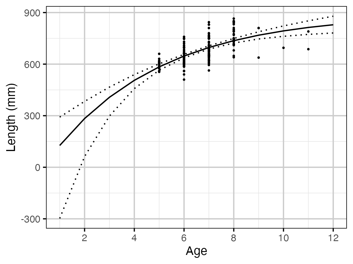
Figure 7. Estimated Rainbow Trout length by age (with 95% CIs).
Condition
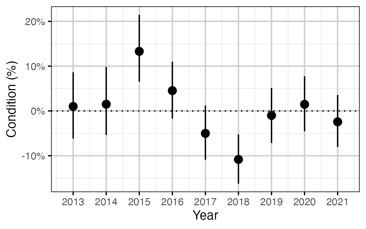
Figure 8. The percent change in the body weight of a 500 mm Rainbow Trout relative to a typical year, by year (with 95% CRIs).
Survival
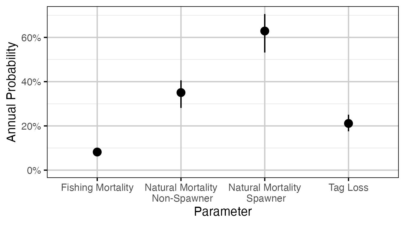
Figure 9. The estimated annual interval probabilities (with 95% CIs).
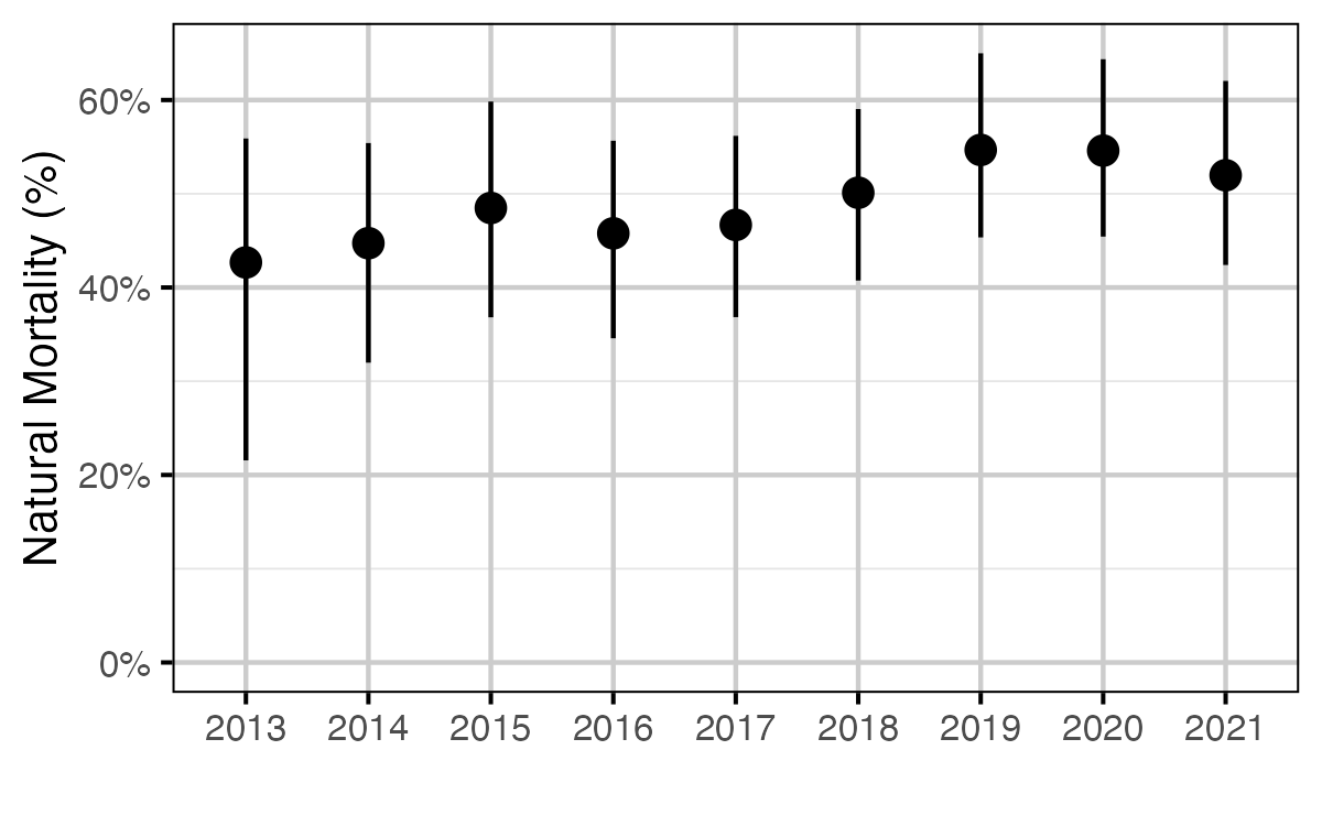
Figure 10. The estimated annual effect on natural mortality (with 95% CRIs).
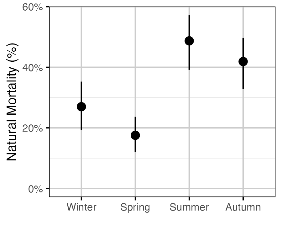
Figure 11. The estimated seasonal effect on natural mortality (with 95% CRIs).
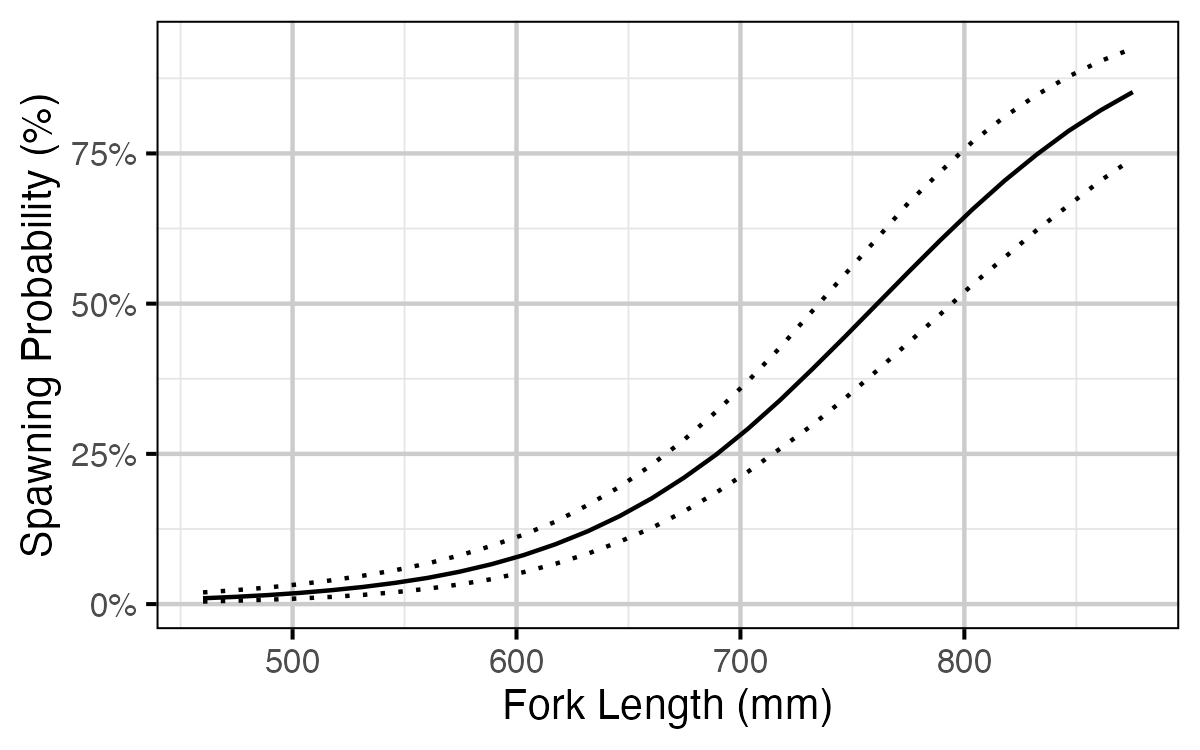
Figure 12. The estimated effect of fork length on spawning probability (with 95% CRIs).
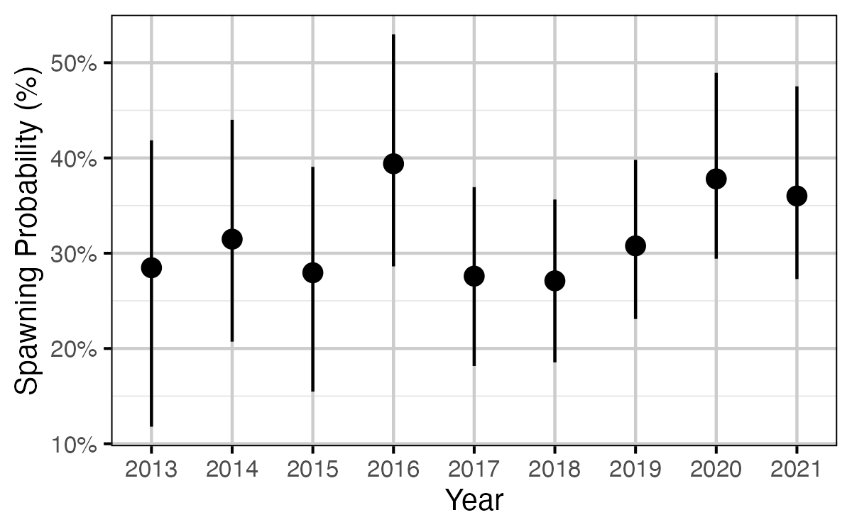
Figure 13. The estimated annual effect on spawning probability for a fish of typical fork length (with 95% CRIs).
Yield-per-Recruit
Slot Limit
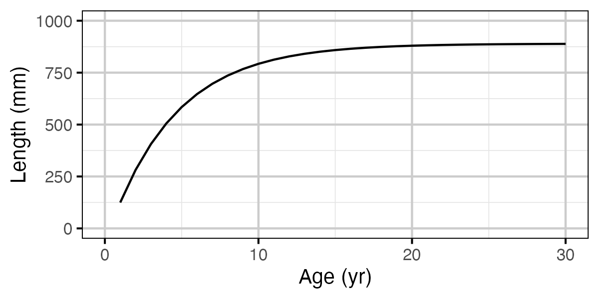
Figure 14. Calculated length by age.
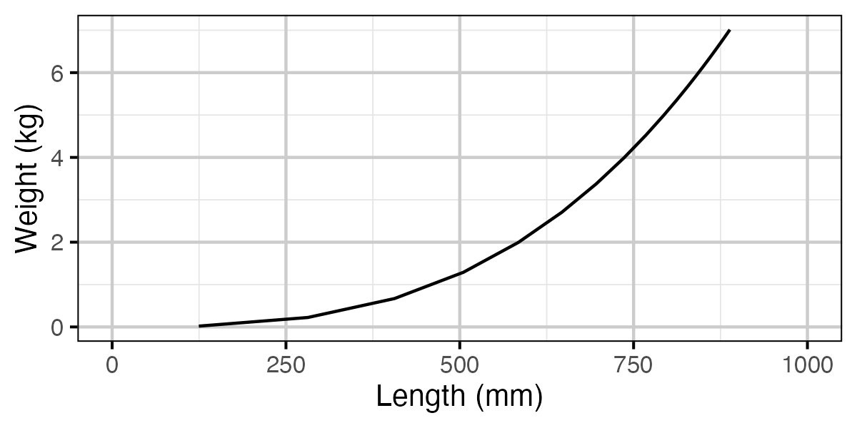
Figure 15. Calculated weight by length.
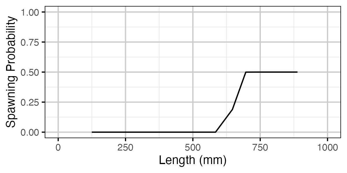
Figure 16. Calculated probability of spawning by length.
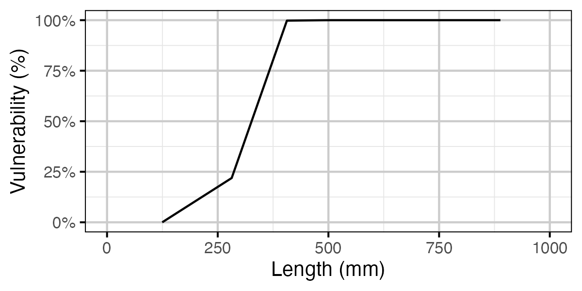
Figure 17. Calculated vulnerability to capture by length.
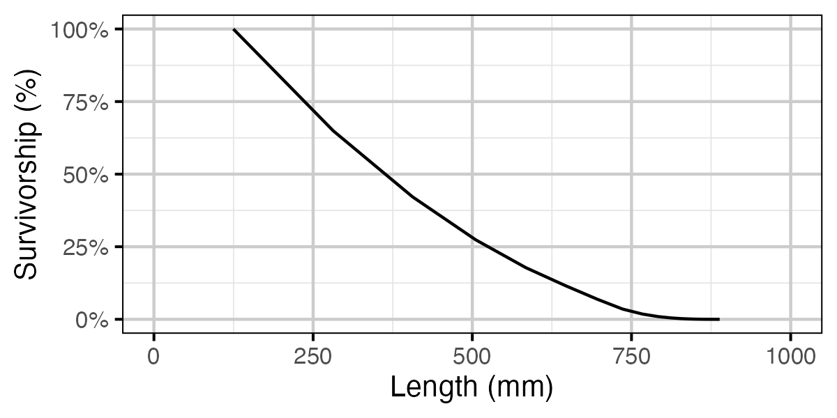
Figure 18. Calculated natural survivorship by length.
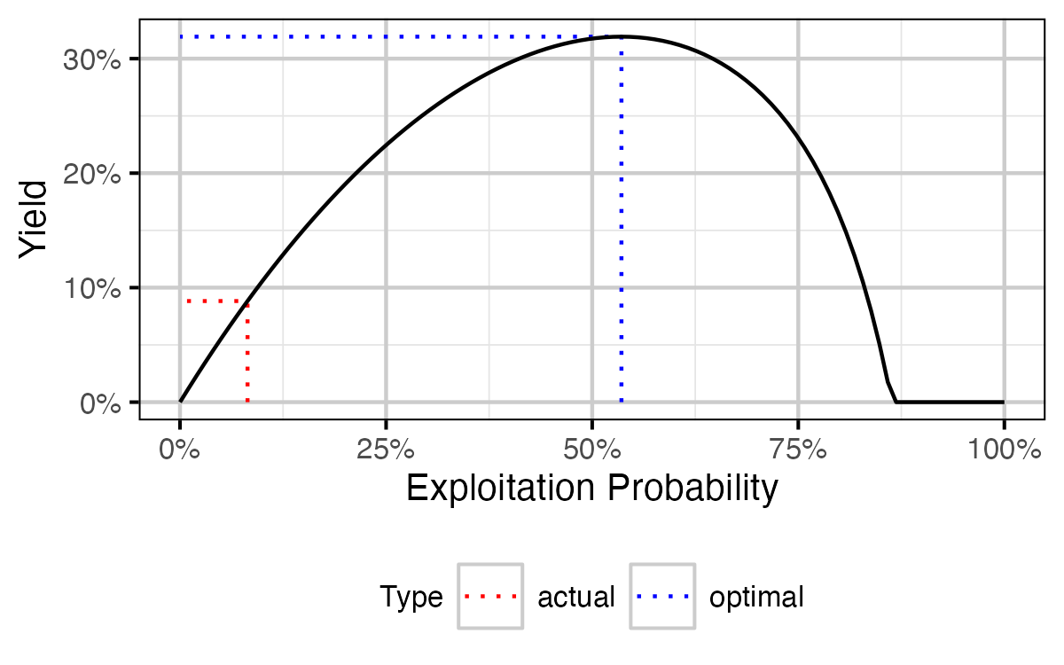
Figure 19. Calculated yield as percent of total unfished biomass by annual interval exploitation rate.
No Slot Limit
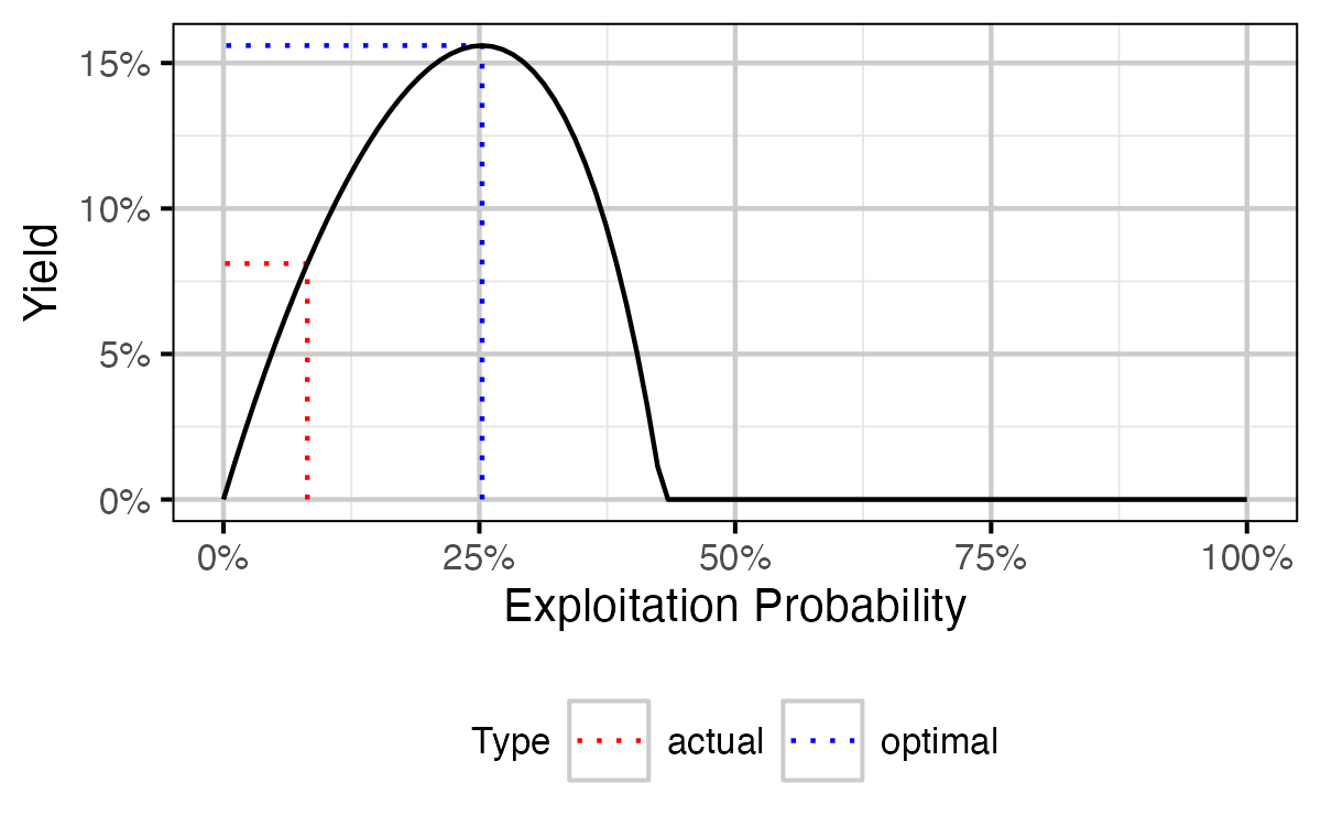
Figure 20. Calculated yield as percent of total unfished biomass by annual interval exploitation rate.
Acknowledgements
The organisations and individuals whose contributions have made this analysis report possible include:
- Quesnel Lake anglers for reporting their catches
- Habitat Conservation Trust Foundation (HCTF)
- and the anglers, hunters, trappers and guides who contribute to the Trust
- Ministry of Forests, Lands and Natural Resource Operations
- Lee Williston
- Mike Ramsay
- Greg Andrusak
- Reel Adventures
- Kerry Reed
- Vicky Lipinski