Mica Tailrace Fish Indexing Study 2013
The suggested citation for this analytic report is:
Thorley, J.L. (2015) Mica Tailrace Fish Indexing Analysis 2013. A Poisson Consulting Analysis Report. URL: https://www.poissonconsulting.ca/f/186605684.
Background
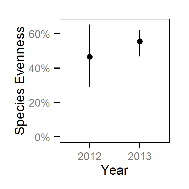
The Mica Tailrace Fish Indexing Study is a four year program to estimate the effects of the addition of two new turbines (Mica 5 and 6) on the ichyofauna and thermal regime in the 2.5 km of the Columbia River downstream of Mica Dam. A single year of fish indexing data (2008) was also available from a previous program. As per the Terms of Reference (TOR) the relative abundance, condition and spatial distribution of the fish populations was assessed. In addition, changes in the species evenness were also estimated.
Methods
Data
The data were provided by the Canadian Columbia River Inter-Tribal Fishery Commission (CCRIFC) in the form of an Access database. All data manipulation was performed using R version 3.0.2 (Team, 2013).
Fish Indexing Data
Individuals were classified as fry (age-0), juvenile (age-1 and older subadults) or adult (sexually mature) based on the following length cut-offs
| Species | Fry | Juvenile |
|---|---|---|
| Bull Trout | < 120 | < 400 |
| Mountain Whitefish | < 120 | < 175 |
| Rainbow Trout | < 120 | < 250 |
| Kokanee | < 100 | < 250 |
Statistical Analysis
Hierarchical Bayesian models were fitted to the data using R version 3.0.2 (Team, 2013) and JAGS 3.3.0 (Plummer, 2012) which interfaced with each other via jaggernaut 1.7 (Thorley, 2014). For additional information on hierarchical Bayesian modelling in the BUGS language, of which JAGS uses a dialect, the reader is referred to Kery and Schaub (2011) pages 41-44.
Unless specified, the models assumed vague (low information) prior distributions (Kéry and Schaub, 2011, p. 36). The posterior distributions were estimated from a minimum of 1,000 Markov Chain Monte Carlo (MCMC) samples thinned from the second halves of three chains (Kéry and Schaub, 2011, pp. 38-40). Model convergence was confirmed by ensuring that Rhat (Kéry and Schaub, 2011, p. 40) was less than 1.1 for each of the parameters in the model (Kéry and Schaub, 2011, p. 61). When possible model adequacy was confirmed by examination of residual plots.
The posterior distributions of the fixed (Kéry and Schaub, 2011, p. 75) parameters are summarised below in terms of a point estimate (mean), lower and upper 95% credible limits (2.5th and 97.5th percentiles), the standard deviation (SD), percent relative error (half the 95% credible interval as a percent of the point estimate) and significance (Kéry and Schaub, 2011, p. 37,42).
The results are displayed graphically by plotting the modeled relationships between particular variables and the response with 95% credible intervals (CRIs) with the remaining variables held constant. In general, continuous and discrete fixed variables are held constant at their mean and first level values respectively while random variables are held constant at their typical values (expected values of the underlying hyperdistributions) (Kéry and Schaub, 2011, pp. 77-82). Where informative the influence of particular variables is expressed in terms of the effect size (i.e., percent change in the response variable) with 95% credible intervals (Bradford et al. 2005). Through the report bull trout data and estimates are plotted in black while rainbow trout are plotted in red. Plots were produced using the ggplot2 R package (Wickham, 2009).
Body Condition
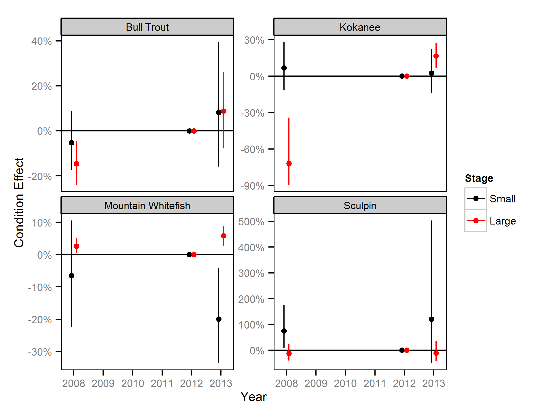
The annual variation in condition (body weight when accounting for body length) was estimated from the boat and backpack electrofishing captures using a mass-length model (He et al. 2008).
Key assumptions of the condition model include:
- Weight varies with body length as an allometric relationship, i.e., \(W = \alpha L^{\beta}\).
- \(\alpha\) varies with year.
- \(\beta\) varies with year.
- The residual variation in weight is log-normally distributed.
Preliminary analyses indicated that site and day of the year were not informative predictors of condition.
Relative Abundance
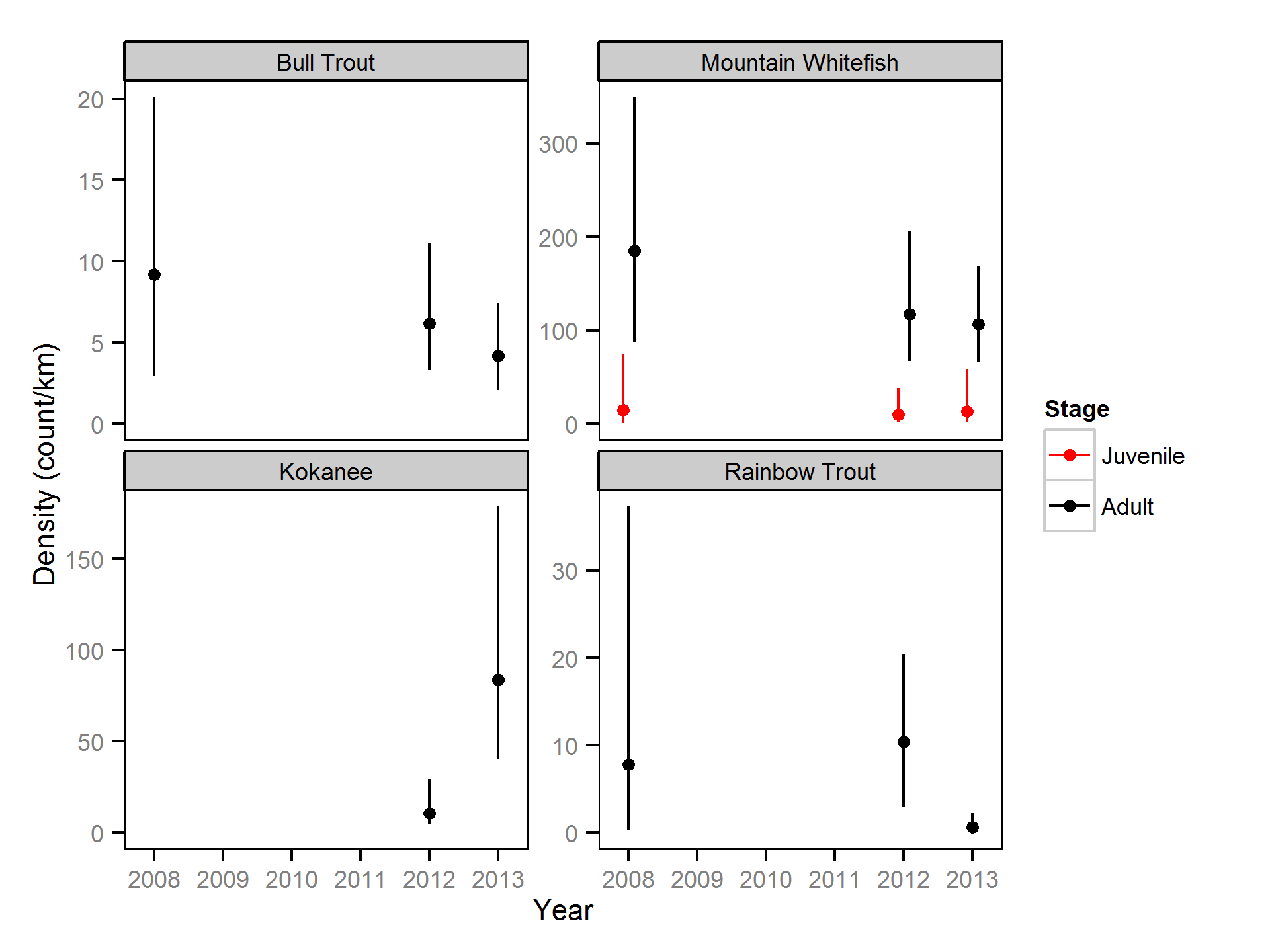
The annual variation in relative abundance was estimated from the boat count and catch data using an over-dispersed Poisson model (Kéry, 2010; Kéry and Schaub, 2011, pp. 168-170,180 and 55-56). Lineal densities are by kilometre of river (as opposed to kilometre of bank).
Key assumptions of the relative abundance model include:
- Lineal density varies with year.
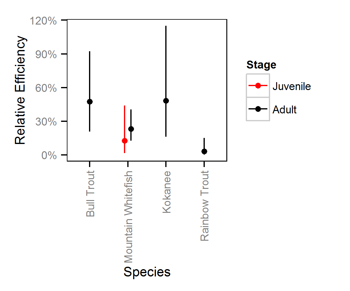
- Lineal catch density is a fixed proportion of lineal count density.
- Expected counts (and catches) are the product of the count (catch) density and the length of river (half the length of bank) sampled.
- Observed counts (and catches) are described by a Poisson-gamma distribution.
Preliminary analyses indicated that site was not an informative predictor of lineal density.
The model does not distinguish between the abundance and observer efficiency, i.e., it estimates the count which is the product of the two. As such it is necessary to assume that changes in observer efficiency by year are negligible in order to interpret the estimates as relative abundance.
Species Evenness
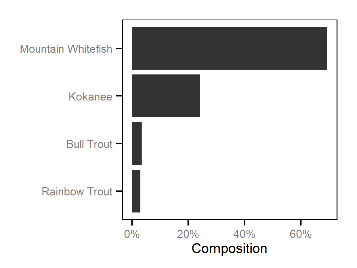
The shannon index of evenness (\(E\)) was calculated from the relative abundance analyses for the adult salmonids using the following formula where \(S\) is the number of species (in this case four) and \(p_i\) is the proportion of the sum of the relative abundances belonging to the ith species.
\[ E = \frac{-\sum p_i \log(p_i)}{ln(S)}\]
Model Code
The first three tables describe the JAGS distributions, functions and operators used in the models. For additional information on the JAGS dialect of the BUGS language see the JAGS User Manual (Plummer, 2012).
JAGS Distributions
| Distribution | Description |
|---|---|
dgamma(shape, rate) |
Gamma distribution |
dlnorm(mu, sd^-2) |
Log-normal distribution |
dnorm(mu, sd^-2) |
Normal distribution |
dpois(lambda) |
Poisson distribution |
dunif(a, b) |
Uniform distribution |
JAGS Functions
| Function | Description |
|---|---|
length(x) |
Length of vector x |
log(x) |
Natural logarithm of x |
JAGS Operators
| Operator | Description |
|---|---|
<- |
Deterministic relationship |
~ |
Stochastic relationship |
1:n |
Vector of integers from 1 to n |
a[1:n] |
Subset of first n values in a |
for (i in 1:n) {...} |
Repeat … for 1 to n times incrementing i each time |
x^y |
Power where x is raised to the power of y |
Variable and parameter definitions and JAGS model code for the analyses are presented below.
The model code adopts the following naming conventions:
- Data variables are named using upper camel case, i.e., site length is
SiteLength. - The number of levels of a discrete data variable
Factoris referenced bynFactor. - Estimated parameters are named using upper camel case prefixed by a lower case character, i.e.,
bDensityRegime. - The SD of a vector of estimated random effects
bRandomis indicated bysRandom. - Unless stated otherwise all effects are linear.
Body Condition
| Variable/Parameter | Description |
|---|---|
bWeightAlpha |
Intercept for eAlpha |
bWeightAlphaYear[i] |
Effect of ith Year on eAlpha |
bWeightBeta |
Intercept for eBeta |
bWeightBetaYear[i] |
Effect of ith Year on eBeta |
eAlpha[i] |
Predicted allometric intercept (on centred log length) for ith fish |
eBeta[i] |
Predicted allometric slope for ith fish |
eWeight[i] |
Predicted weight of ith fish |
Length[i] |
Centred log Length of ith fish |
sWeight |
SD of residual variation in log(Weight) |
Weight[i] |
Weight of ith fish |
Year[i] |
Year of capture of of ith fish |
Body Condition - Model 1
model{

  bWeightAlpha ~ dnorm(5, 5^-2)
  bWeightBeta ~ dnorm(3, 5^-2)

  bWeightAlphaYear[1] <- 0
  for(i in 2:nYear) {
    bWeightAlphaYear[i] ~ dnorm(0, 2^-2)
  }

  bWeightBetaYear[1] <- 0
  for(i in 2:nYear) {
    bWeightBetaYear[i] ~ dnorm(0, 2^-2)
  }

  sWeight ~ dunif(0, 5)
  for (i in 1:length(Weight)) {
    eWeightAlpha[i] <- bWeightAlpha
                        + bWeightAlphaYear[Year[i]]

    eWeightBeta[i] <- bWeightBeta
                        + bWeightBetaYear[Year[i]]

    log(eWeight[i]) <- eWeightAlpha[i] + eWeightBeta[i] * Length[i]

    Weight[i] ~ dlnorm(log(eWeight[i]), sWeight^-2)
  }
}
Relative Abundance
| Variable/Parameter | Description |
|---|---|
bDensity |
Intercept for log(eDensity) |
bDensityYear[i] |
Effect of ith Year on log(eDensity) |
bEfficiencyVisitType[i] |
Value of log(eEfficiency) for ith VisitType |
Count[i] |
Number of fish counted or captured on ith site visit |
eAbundance[i] |
Predicted relative abundance for ith site visit |
eDensity[i] |
Predicted relative lineal density for ith site visit |
eDispersion[i] |
Predicted over-dispersion for ith site visit |
eEfficiency[i] |
Predicted efficiency relative to counting for ith site visit |
sDispersion |
SD of eDispersion |
SiteLength[i] |
Length of bank surveyed on ith site visit |
VisitType[i] |
Type of ith site visit, i.e., count versus catch |
Year[i] |
Year of ith site visit |
Relative Abundance - Model 1
model{

  bEfficiencyVisitType[1] <- 0
  for (i in 2:nVisitType) {
    bEfficiencyVisitType[i] ~ dnorm(0, 2^-2)
  }

  bDensity ~ dnorm(0, 5^-2)

  bDensityYear[1] <- 0
  for(i in 2:nYear) {
    bDensityYear[i] ~ dnorm(0, 5^-2)
  }

  sDispersion ~ dunif(0, 5)
  for (i in 1:length(Year)) {

    log(eEfficiency[i]) <- bEfficiencyVisitType[VisitType[i]]

    log(eDensity[i]) <- bDensity
                          + bDensityYear[Year[i]]

    eAbundance[i] <- eDensity[i] * SiteLength[i] / 2

    eDispersion[i] ~ dgamma(1 / sDispersion^2, 1 / sDispersion^2)
    Count[i] ~ dpois(eAbundance[i] * eEfficiency[i] * eDispersion[i])
  }
}
Parameter Estimates
The posterior distributions for the fixed (Kery and Schaub 2011 p. 75) parameters in each model are summarised below.
Body Condition - Bull Trout
| Parameter | Estimate | Lower | Upper | SD | Error | Significance |
|---|---|---|---|---|---|---|
| bWeightAlpha | 6.6663 | 6.62297 | 6.7071 | 0.02126 | 1 | 0.0000 |
| bWeightAlphaYear[2] | 0.1110 | 0.02351 | 0.1898 | 0.04266 | 75 | 0.0107 |
| bWeightAlphaYear[3] | 0.1870 | 0.05888 | 0.3140 | 0.06467 | 68 | 0.0040 |
| bWeightBeta | 3.0549 | 2.92265 | 3.1858 | 0.06722 | 4 | 0.0000 |
| bWeightBetaYear[2] | 0.1476 | -0.11745 | 0.4231 | 0.14284 | 183 | 0.3067 |
| bWeightBetaYear[3] | 0.1628 | -0.24565 | 0.5931 | 0.20786 | 258 | 0.4440 |
| sWeight | 0.1660 | 0.14380 | 0.1928 | 0.01255 | 15 | 0.0000 |
| Rhat | Iterations |
|---|---|
| 1.05 | 1000 |
Body Condition - Kokanee
| Parameter | Estimate | Lower | Upper | SD | Error | Significance |
|---|---|---|---|---|---|---|
| bWeightAlpha | 3.7258 | 3.0774 | 4.4352 | 0.347120 | 18 | 0 |
| bWeightAlphaYear[2] | 0.9481 | 0.2396 | 1.5962 | 0.349190 | 72 | 0 |
| bWeightAlphaYear[3] | 1.0612 | 0.3473 | 1.7041 | 0.349320 | 64 | 0 |
| bWeightBeta | 2.3539 | 1.8540 | 2.8981 | 0.273610 | 22 | 0 |
| bWeightBetaYear[2] | 0.9756 | 0.4257 | 1.4835 | 0.275000 | 54 | 0 |
| bWeightBetaYear[3] | 1.0646 | 0.5188 | 1.5771 | 0.277360 | 50 | 0 |
| sWeight | 0.1989 | 0.1808 | 0.2177 | 0.009798 | 9 | 0 |
| Rhat | Iterations |
|---|---|
| 2.48 | 8000 |
Body Condition - Mountain Whitefish
| Parameter | Estimate | Lower | Upper | SD | Error | Significance |
|---|---|---|---|---|---|---|
| bWeightAlpha | 5.30073 | 5.28951 | 5.31227 | 0.005996 | 0 | 0.0000 |
| bWeightAlphaYear[2] | -0.02928 | -0.05159 | -0.00839 | 0.011308 | 74 | 0.0093 |
| bWeightAlphaYear[3] | 0.03649 | 0.01065 | 0.06238 | 0.013181 | 71 | 0.0040 |
| bWeightBeta | 3.09222 | 3.04021 | 3.14160 | 0.026296 | 2 | 0.0000 |
| bWeightBetaYear[2] | -0.08493 | -0.23357 | 0.05644 | 0.073012 | 171 | 0.2280 |
| bWeightBetaYear[3] | 0.16362 | 0.07622 | 0.25032 | 0.046251 | 53 | 0.0000 |
| sWeight | 0.11210 | 0.10560 | 0.11907 | 0.003466 | 6 | 0.0000 |
| Rhat | Iterations |
|---|---|
| 1.01 | 1000 |
Body Condition - Sculpin
| Parameter | Estimate | Lower | Upper | SD | Error | Significance |
|---|---|---|---|---|---|---|
| bWeightAlpha | 0.60805 | 0.44454 | 0.7623 | 0.08052 | 26 | 0.0000 |
| bWeightAlphaYear[2] | -0.08973 | -0.34894 | 0.1815 | 0.13498 | 296 | 0.5133 |
| bWeightAlphaYear[3] | 0.02680 | -0.41144 | 0.4415 | 0.21587 | 1591 | 0.8880 |
| bWeightBeta | 2.01672 | 1.42554 | 2.5854 | 0.29212 | 29 | 0.0000 |
| bWeightBetaYear[2] | 0.74049 | 0.06063 | 1.4480 | 0.35404 | 94 | 0.0320 |
| bWeightBetaYear[3] | -0.05337 | -1.63674 | 1.5873 | 0.81467 | 3020 | 0.9320 |
| sWeight | 0.41920 | 0.34300 | 0.5119 | 0.04351 | 20 | 0.0000 |
| Rhat | Iterations |
|---|---|
| 1.01 | 2000 |
Relative Abundance - Bull Trout - Adult
| Parameter | Estimate | Lower | Upper | SD | Error | Significance |
|---|---|---|---|---|---|---|
| bDensity | -4.1543 | -5.1693 | -3.25991 | 0.4803 | 23 | 0.0000 |
| bDensityYear[2] | -0.3369 | -1.1760 | 0.57849 | 0.4493 | 260 | 0.4491 |
| bDensityYear[3] | -0.7237 | -1.6146 | 0.27099 | 0.4818 | 130 | 0.1257 |
| bEfficiencyVisitType[2] | -0.8194 | -1.5697 | -0.08067 | 0.3883 | 91 | 0.0399 |
| sDispersion | 0.6178 | 0.3101 | 0.98243 | 0.1679 | 54 | 0.0000 |
| Rhat | Iterations |
|---|---|
| 1.04 | 10000 |
Relative Abundance - Kokanee - Adult
| Parameter | Estimate | Lower | Upper | SD | Error | Significance |
|---|---|---|---|---|---|---|
| bDensity | -4.0264 | -4.8106 | -2.8808 | 0.4722 | 24 | 0.0000 |
| bDensityYear[2] | 2.1117 | 1.1227 | 3.1958 | 0.5078 | 49 | 0.0000 |
| bEfficiencyVisitType[2] | -0.8493 | -1.8183 | 0.1401 | 0.5014 | 115 | 0.1101 |
| sDispersion | 1.0093 | 0.7081 | 1.3934 | 0.1855 | 34 | 0.0000 |
| Rhat | Iterations |
|---|---|
| 1.04 | 20000 |
Relative Abundance - Mountain Whitefish - Adult
| Parameter | Estimate | Lower | Upper | SD | Error | Significance |
|---|---|---|---|---|---|---|
| bDensity | -1.1009 | -1.7849 | -0.4046 | 0.35218 | 63 | 0.0019 |
| bDensityYear[2] | -0.4333 | -1.0253 | 0.1731 | 0.30816 | 138 | 0.1595 |
| bDensityYear[3] | -0.5189 | -1.1470 | 0.1345 | 0.32841 | 123 | 0.1026 |
| bEfficiencyVisitType[2] | -1.5020 | -2.0758 | -0.9049 | 0.29297 | 39 | 0.0000 |
| sDispersion | 0.6197 | 0.4653 | 0.8134 | 0.08966 | 28 | 0.0000 |
| Rhat | Iterations |
|---|---|
| 1.03 | 40000 |
Relative Abundance - Mountain Whitefish - Juvenile
| Parameter | Estimate | Lower | Upper | SD | Error | Significance |
|---|---|---|---|---|---|---|
| bDensity | -4.20980 | -6.343 | -1.9485 | 1.1265 | 52 | 0.0000 |
| bDensityYear[2] | -0.06503 | -2.405 | 2.1444 | 1.1877 | 3498 | 0.9700 |
| bDensityYear[3] | 0.11825 | -1.921 | 2.1892 | 1.0555 | 1738 | 0.9314 |
| bEfficiencyVisitType[2] | -2.43930 | -4.201 | -0.8194 | 0.8690 | 69 | 0.0058 |
| sDispersion | 1.77201 | 1.154 | 2.5978 | 0.3799 | 41 | 0.0000 |
| Rhat | Iterations |
|---|---|
| 1.03 | 20000 |
Relative Abundance - Rainbow Trout - Adult
| Parameter | Estimate | Lower | Upper | SD | Error | Significance |
|---|---|---|---|---|---|---|
| bDensity | -4.9413 | -7.4493 | -2.6395 | 1.2654 | 49 | 0.0000 |
| bDensityYear[2] | 0.6820 | -1.6920 | 3.1542 | 1.2903 | 355 | 0.6327 |
| bDensityYear[3] | -2.2282 | -5.0568 | 0.8387 | 1.5161 | 132 | 0.1437 |
| bEfficiencyVisitType[2] | -3.9713 | -5.9724 | -1.8908 | 1.0204 | 51 | 0.0000 |
| sDispersion | 0.9266 | 0.2585 | 2.2490 | 0.5351 | 107 | 0.0000 |
| Rhat | Iterations |
|---|---|
| 1.07 | 10000 |
Figures
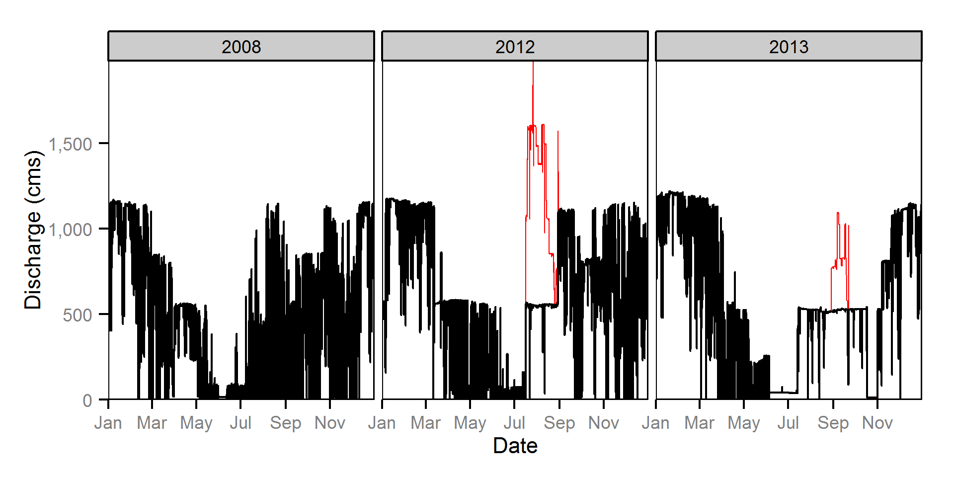
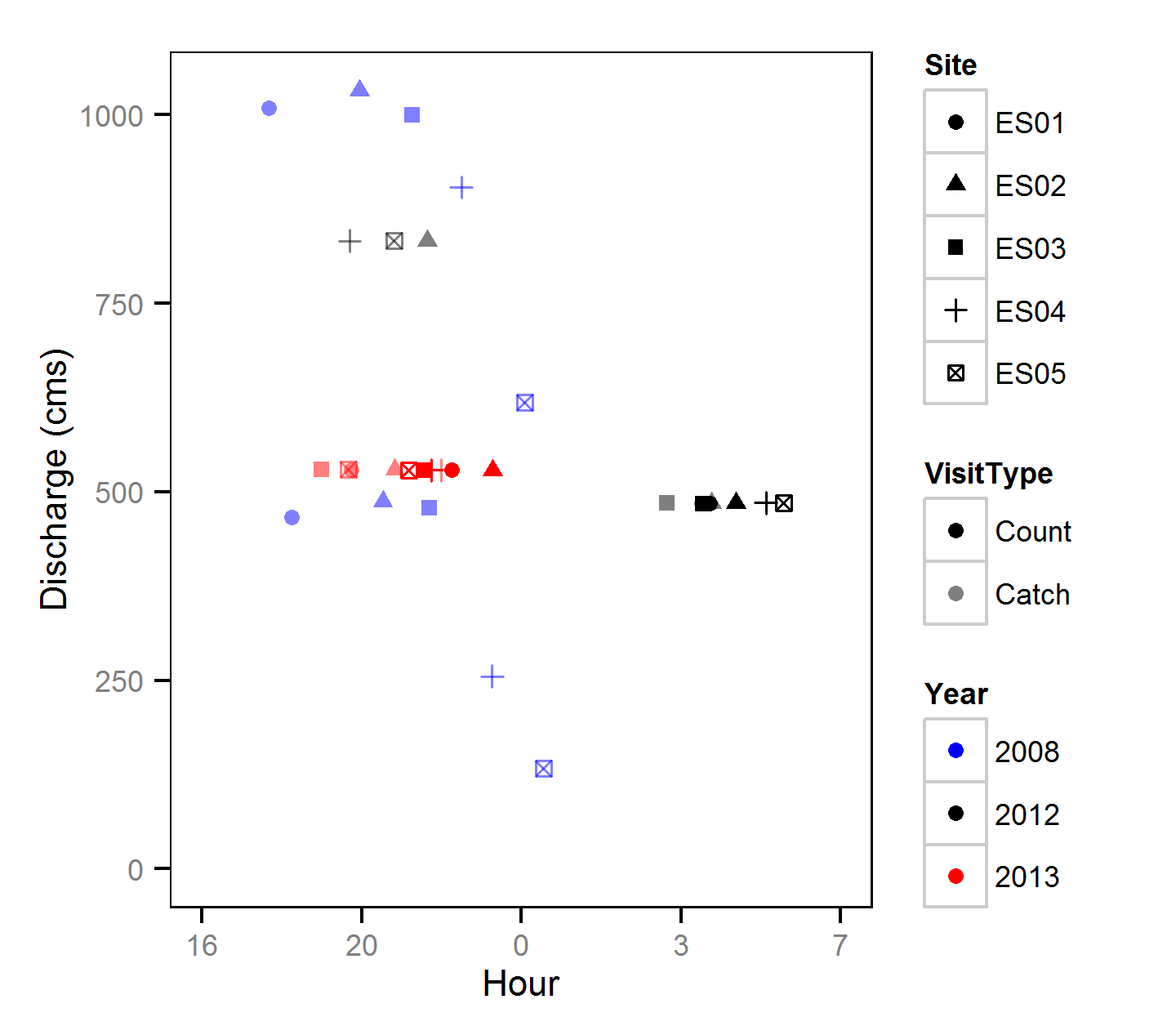
Discharge
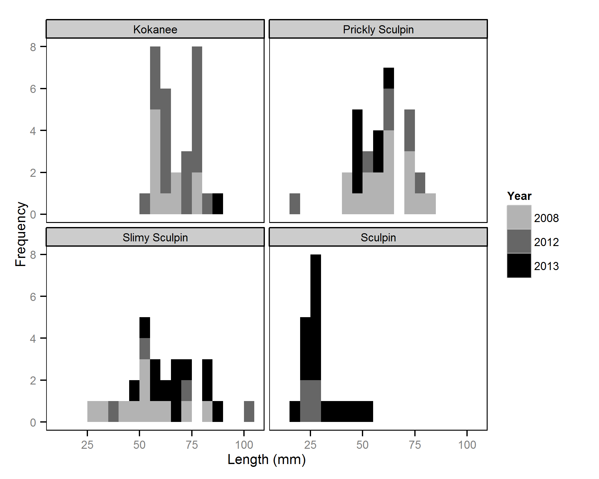
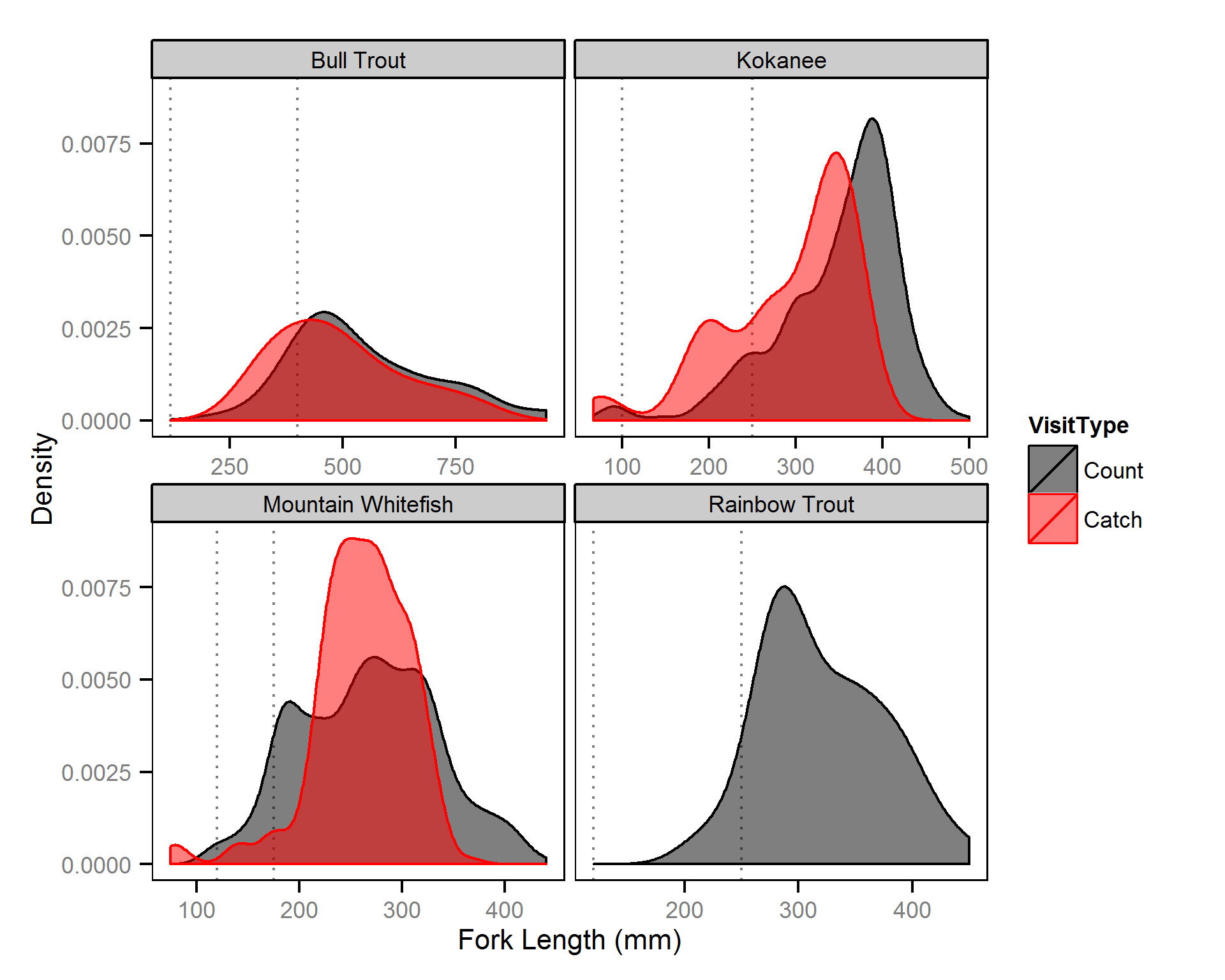
Length
Body Condition
Relative Abundance
Spatial Distribution - Bull Trout - Adult
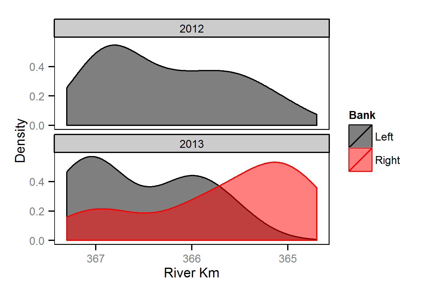
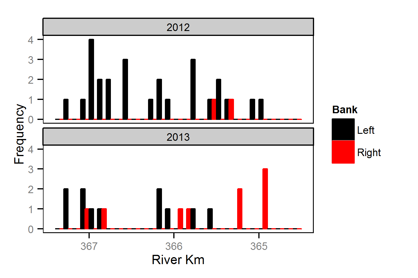
Spatial Distribution - Kokanee - Adult
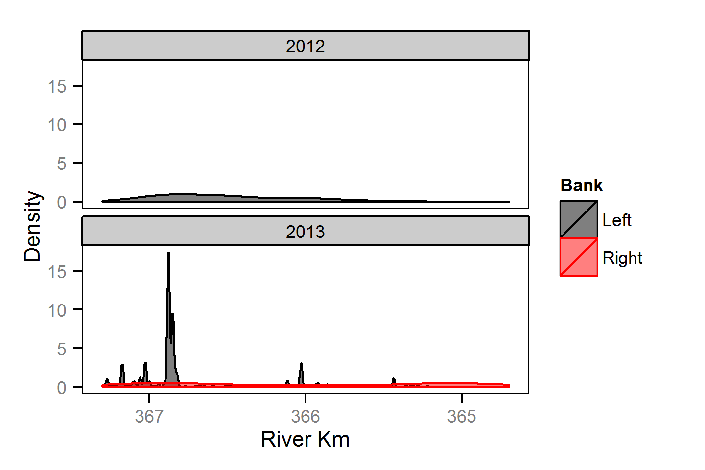
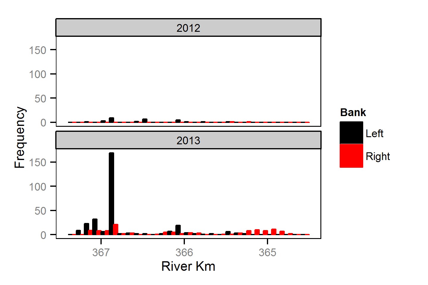
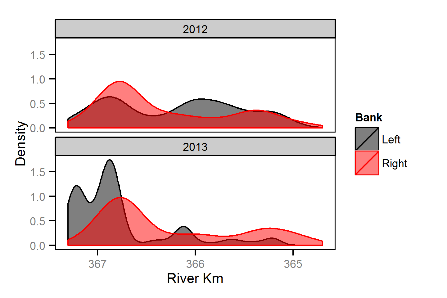
Spatial Distribution - Mountain Whitefish - Adult
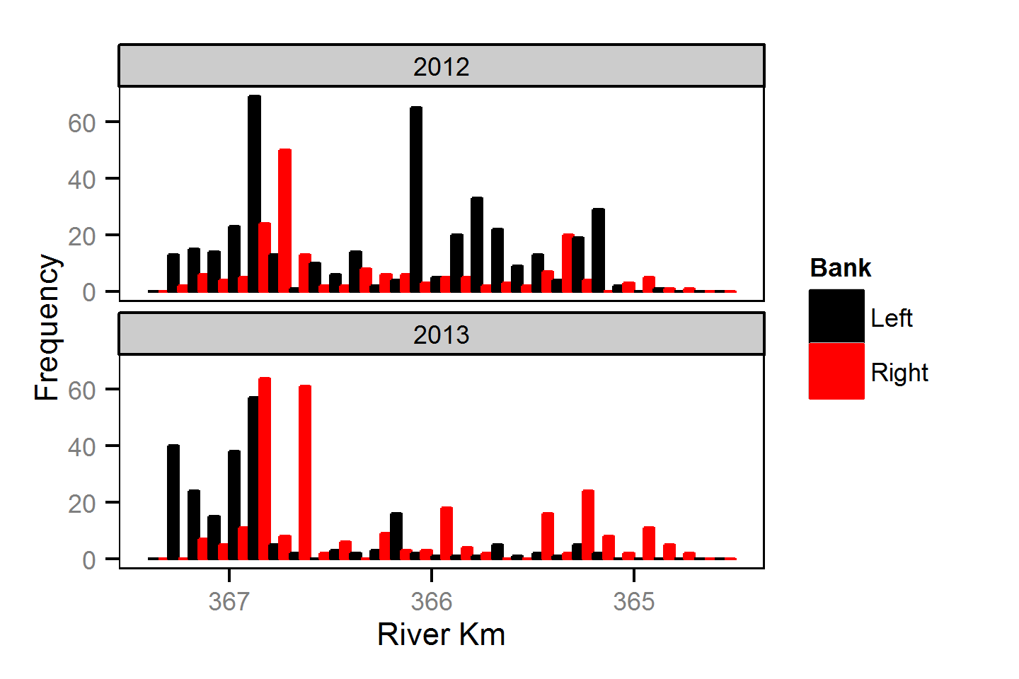
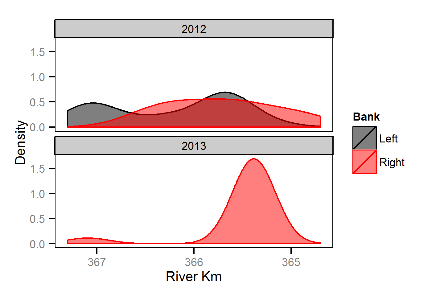
Spatial Distribution - Mountain Whitefish - Juvenile
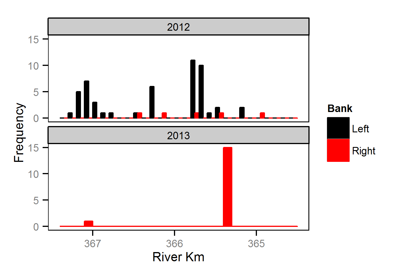
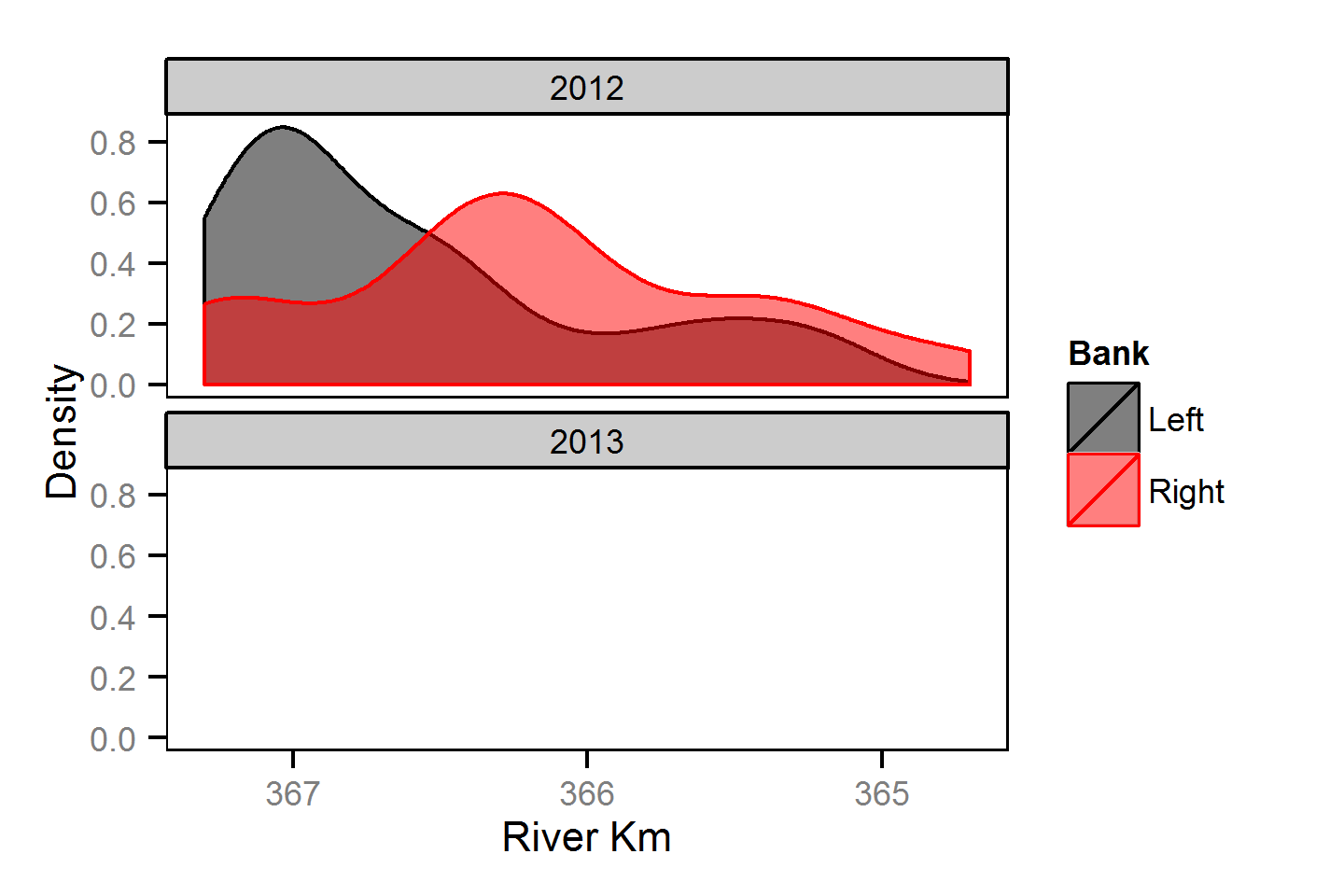
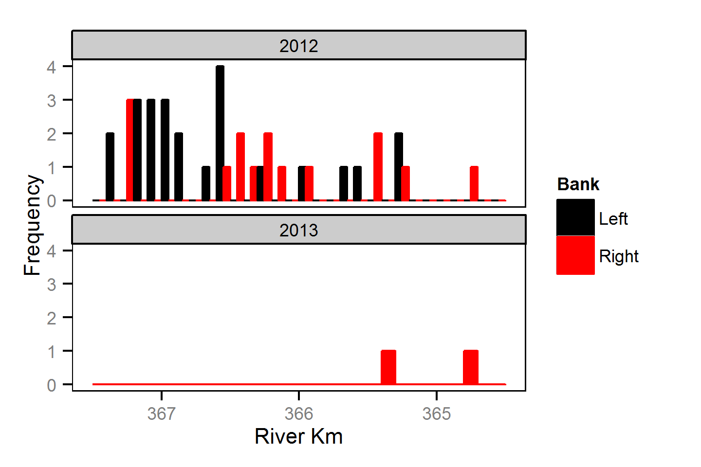
Spatial Distribution - Rainbow Trout - Adult
References
- Michael Bradford, Josh Korman, Paul Higgins, (2005) Using confidence intervals to estimate the response of salmon populations (Oncorhynchus spp.) to experimental habitat alterations. Canadian Journal of Fisheries and Aquatic Sciences 62 (12) 2716-2726 10.1139/f05-179
- Hadley Wickham, (2009) ggplot2: elegant graphics for data analysis. http://had.co.nz/ggplot2/book
- Ji He, James Bence, James Johnson, David Clapp, Mark Ebener, (2008) Modeling Variation in Mass-Length Relations and Condition Indices of Lake Trout and Chinook Salmon in Lake Huron: A Hierarchical Bayesian Approach. Transactions of the American Fisheries Society 137 (3) 801-817 10.1577/T07-012.1
- Joseph Thorley, (2014) jaggernaut: An R package to facilitate Bayesian analyses using JAGS (Just Another Gibbs Sampler). https://github.com/joethorley/jaggernaut
- Marc Kéry, Michael Schaub, (2011) Bayesian population analysis using {WinBUGS} : a hierarchical perspective. http://www.vogelwarte.ch/bpa.html
- Marc Kéry, (2010) Introduction to {WinBUGS} for Ecologists: A Bayesian approach to regression, {ANOVA}, mixed models and related analyses. http://public.eblib.com/EBLPublic/PublicView.do?ptiID=629953
- Martyn Plummer, (2012) {JAGS} version 3.3.0 user manual. http://sourceforge.net/projects/mcmc-jags/files/Manuals/3.x/
- R Team, (2013) R: a language and environment for statistical computing. http://www.R-project.org
Acknowledgements
The organisations and individuals whose contributions have made this analysis report possible include:
- BC Hydro
- Jason Watson
- Margo Dennis
- Guy Martel
- Alf Leake
- Karen Bray
- Peter McCann
- Fred Katunar
- Columbia River Inter-Tribal Fisheries Commission (CCRIFC)
- Jon Bisset
- Will Warnock
- JoAnne Fisher
- Jim Clarricoates
- Jose Galdamez
- Bill Green
- Applied Aquatic Research (AAR)
- Tom Boag
- Matt Sparrow
- Poisson Consulting
- Robyn Irvine
- Thomas Resources
- Mark Thomas
- Ministry of Forests, Lands and Natural Resource Operations (MFLNRO)
- Albert Chirico
- Gary Pavan