Mica Dam Expansion Water Temperature and Fish Indexing Study 2020
The suggested citation for this analytic appendix is:
Thorley, J.L. & Amies-Galonski, E. (2021) Mica Dam Expansion Water Temperature and Fish Indexing Study 2020. A Poisson Consulting Analysis Appendix. URL: https://www.poissonconsulting.ca/f/955630057.
Background
The Mica Tailrace Fish Indexing Study is a multi-year program to estimate the effects of the addition of two new turbines (Mica 5 and 6) on the ichyofauna and thermal regime in the 2.5 km of the Columbia River downstream of Mica Dam. A single year of fish indexing data (2008) was also available from a previous program. As per the Terms of Reference (TOR) the relative abundance, condition and spatial distribution of the fish populations was assessed.
Mica 5 became operational on January 28th 2015 and Mica 6 became operational on December 22nd 2015.
Data Preparation
The fish and downstream temperature data were provided by the Ktunaxa Nation. The discharge and elevation data were queried from the Columbia Basin Hydrological Database.
The data were cleaned and tidied using R version 4.0.5 (R Core Team 2020).
Length Cutoffs
Individuals were classified as fry (age-0), juvenile (age-1 and older subadults) or adult (sexually mature) based on the length cut-offs in Table 1.
Statistical Analysis
Model parameters were estimated using Bayesian methods. The estimates were produced using JAGS (Plummer 2003). For additional information on Bayesian estimation the reader is referred to McElreath (2016).
Unless stated otherwise, the Bayesian analyses used weakly informative normal and half-normal prior distributions (Gelman, Simpson, and Betancourt 2017). The posterior distributions were estimated from 1500 Markov Chain Monte Carlo (MCMC) samples thinned from the second halves of 3 chains (Kery and Schaub 2011, 38–40). Model convergence was confirmed by ensuring that the potential scale reduction factor \(\hat{R} \leq 1.05\) (Kery and Schaub 2011, 40) and the effective sample size (Brooks et al. 2011) \(\textrm{ESS} \geq 150\) for each of the monitored parameters (Kery and Schaub 2011, 61).
The parameters are summarised in terms of the point estimate, lower and upper 95% credible limits (CLs) and the surprisal s-value (Greenland 2019). The estimate is the median (50th percentile) of the MCMC samples while the 95% CLs are the 2.5th and 97.5th percentiles. The s-value can be considered a test of directionality. More specifically it indicates how surprising (in bits) it would be to discover that the true value of the parameter is in the opposite direction to the estimate. An s-value of 4.3 bits, which is equivalent to a p-value (Kery and Schaub 2011; Greenland and Poole 2013) of 0.05, indicates that the surprise would be equivalent to throwing 4.3 heads in a row. The requirement that non-essential explanatory variables have s-values \(\geq\) 4.3 bits provides a useful model selection heuristic (Kery and Schaub 2011).
The results are displayed graphically by plotting the modeled relationships between particular variables and the response(s) with the remaining variables held constant. In general, continuous and discrete fixed variables are held constant at their mean and first level values, respectively, while random variables are held constant at their typical values (expected values of the underlying hyperdistributions) (Kery and Schaub 2011, 77–82). When informative the influence of particular variables is expressed in terms of the effect size (i.e., percent or n-fold change in the response variable) with 95% credible intervals (CIs, Bradford, Korman, and Higgins 2005).
The analyses were implemented using R version 4.0.5
(R Core Team 2020) and the
mbr family of packages.
Model Descriptions
Body Condition
The annual variation in condition (body weight when accounting for body length) was estimated from the boat and backpack electrofishing captures using a mass-length model (He et al. 2008).
Key assumptions of the condition model include:
- Weight varies with body length as an allometric relationship, i.e., \(W = \alpha L^{\beta}\).
- \(\alpha\) varies randomly with year.
- \(\alpha\) varies by period (pre versus post Mica 5 and 6).
- The residual variation in weight is log-normally distributed.
Preliminary analyses indicated that site and day of the year were not informative predictors of condition.
Relative Abundance
The annual variation in relative abundance was estimated from the boat count and catch data using an over-dispersed Poisson model (Kery and Schaub 2011). Lineal densities are by kilometre of river (as opposed to kilometre of bank).
Key assumptions of the relative abundance model include:
- Lineal count density varies by period.
- Lineal count density varies randomly with year.
- Lineal catch efficiency is a fixed multiplier of lineal count efficiency.
- Expected counts (and catches) are the product of the count (catch) density and the length of river (half the length of bank) sampled.
- Observed counts (and catches) are described by a Poisson-gamma distribution.
Preliminary analyses indicated that site and discharge were not informative predictors of the lineal count (or catch) density.
The model does not distinguish between the abundance and observer efficiency, i.e., it estimates the count which is the product of the two. As such it is necessary to assume that changes in observer efficiency by year are negligible in order to interpret the estimates as relative abundance.
Water Temperature
Tailrace
Climatic variation can cause large differences in annual temperatures. Consequently, we explored the data for an effect of the additional turbines on the difference in the water temperature between the right versus left bank and when moving downstream. All apparent systematic differences were within the accuracy of the temperature loggers (\(\pm 0.2^{\circ}\text{C}\)).
Forebay and Tailrace
In 2020 the BC Hydro thermistor data for the Mica Dam forebay were analysed using Maximum Likelihood (Millar 2011) and TMB (Kristensen et al. 2016) to determine the extent to which discharge from the turbines and the air temperature influences the water temperature in the tailrace.
Key assumptions of the hourly temperature model include:
- The effective depth of each unit depends on the unit (as a random effect) and its discharge (as a fixed effect).
- The water temperature effect of each unit depends on its effective depth and the stratification in the forebay.
- The water temperature is affected by release from the dam and the difference in air temperature and the water temperature.
- The temporal autocorrelation is described a first order moving average process.
- The residual water temperature at the tailrace temperature logger is normally distributed.
Despite the incorporation of a first order moving average process the residual variation in the hourly tailrace water temperature was strongly autocorrelated. Consequently CIs are not provided for the coefficients or estimates.
Model Templates
Condition
.model{
  bAlpha ~ dnorm(5, 2^-2)
  bBeta ~ dnorm(3, 2^-2)

  bAlphaPeriod[1] <- 0
  for(i in 2:nPeriod) {
    bAlphaPeriod[i] ~ dnorm(0, 2^-2)
  }

  sAlphaAnnual ~ dnorm(0, 2^-2) T(0,)
  for(i in 1:nAnnual) {
    bAlphaAnnual[i] ~ dnorm(0, sAlphaAnnual^-2)
  }

  sWeight ~ dnorm(0, 2^-2) T(0,)
  for (i in 1:length(Weight)) {
    eAlpha[i] <- bAlpha + bAlphaPeriod[Period[i]] + bAlphaAnnual[Annual[i]]
    eBeta[i] <- bBeta
    log(eWeight[i]) <- eAlpha[i] + eBeta[i] * Length[i]
    Weight[i] ~ dlnorm(log(eWeight[i]), sWeight^-2)
  }
Block 1.
Relative Abundance
.model{
  bEfficiencyVisitType[1] <- 0
  for (i in 2:nVisitType) {
    bEfficiencyVisitType[i] ~ dnorm(0, 1^-2)
  }

  bDensity ~ dnorm(0, 5^-2)

  bDensityPeriod[1] <- 0
  for(i in 2:nPeriod) {
    bDensityPeriod[i] ~ dnorm(0, 2^-2)
  }

  sDensityAnnual ~ dnorm(0, 2^-2) T(0, )
  for(i in 1:nAnnual) {
    bDensityAnnual[i] ~ dnorm(0, sDensityAnnual^-2)
  }

  sDispersion ~ dnorm(0, 2^-2) T(0, )
  for (i in 1:length(Annual)) {
    log(eEfficiency[i]) <- bEfficiencyVisitType[VisitType[i]]
    log(eDensity[i]) <- bDensity + bDensityPeriod[Period[i]] + bDensityAnnual[Annual[i]]
    eAbundance[i] <- eDensity[i] * SiteLength[i] / 2
    eDispersion[i] ~ dgamma(1 / sDispersion^2, 1 / sDispersion^2)
    Count[i] ~ dpois(eAbundance[i] * eEfficiency[i] * eDispersion[i])
  }
Block 2.
Forebay and Tailrace
.#include <TMB.hpp>

template<class Type>
Type objective_function<Type>::operator() () {

DATA_VECTOR(Tailrace);
DATA_VECTOR(Intake);
DATA_VECTOR(Forebay);
DATA_VECTOR(Air);
DATA_VECTOR(Unit1);
DATA_VECTOR(Unit2);
DATA_VECTOR(Unit3);
DATA_VECTOR(Unit4);
DATA_VECTOR(Unit5);
DATA_VECTOR(Unit6);
DATA_VECTOR(Spill);
DATA_IVECTOR(Consecutive);

PARAMETER(sDepthUnit);
PARAMETER_VECTOR(bDepthUnit);
PARAMETER(bDepthSpill0);
PARAMETER_VECTOR(bDepthTurbineUnit);
PARAMETER(bRelease);
PARAMETER(bReleaseAir);
PARAMETER(bRho);
PARAMETER(sTailrace);

vector<Type> eTurbineUnit1 = Tailrace;
vector<Type> eTurbineUnit2 = Tailrace;
vector<Type> eTurbineUnit3 = Tailrace;
vector<Type> eTurbineUnit4 = Tailrace;
vector<Type> eTurbineUnit5 = Tailrace;
vector<Type> eTurbineUnit6 = Tailrace;
vector<Type> eDischarge = Tailrace;
vector<Type> eDepthTurbineUnit1 = Tailrace;
vector<Type> eDepthTurbineUnit2 = Tailrace;
vector<Type> eDepthTurbineUnit3 = Tailrace;
vector<Type> eDepthTurbineUnit4 = Tailrace;
vector<Type> eDepthTurbineUnit5 = Tailrace;
vector<Type> eDepthTurbineUnit6 = Tailrace;
vector<Type> eDepthSpill = Tailrace;
vector<Type> eStratification = Tailrace;
vector<Type> eEffectTurbineUnit1 = Tailrace;
vector<Type> eEffectTurbineUnit2 = Tailrace;
vector<Type> eEffectTurbineUnit3 = Tailrace;
vector<Type> eEffectTurbineUnit4 = Tailrace;
vector<Type> eEffectTurbineUnit5 = Tailrace;
vector<Type> eEffectTurbineUnit6 = Tailrace;
vector<Type> eEffectSpill = Tailrace;
vector<Type> eEffectDischarge = Tailrace;
vector<Type> eReleaseEffect = Tailrace;
vector<Type> eOutput = Tailrace;
vector<Type> eRelease = Tailrace;
vector<Type> eTailrace = Tailrace;

Type nll = 0.0;

eTailrace(0) = Tailrace(0);

for(int i = 0; i < 6; i++){
  nll -= dnorm(bDepthUnit(i), Type(0), exp(sDepthUnit), true);

for(int i = 1; i < Tailrace.size(); i++){
  eTurbineUnit1(i) = Unit1(i) + 0.0001;
  eTurbineUnit2(i) = Unit2(i) + 0.0001;
  eTurbineUnit3(i) = Unit3(i) + 0.0001;
  eTurbineUnit4(i) = Unit4(i) + 0.0001;
  eTurbineUnit5(i) = Unit5(i) + 0.0001;
  eTurbineUnit6(i) = Unit6(i) + 0.0001;
  eDischarge(i) = eTurbineUnit1(i) + eTurbineUnit2(i) + eTurbineUnit3(i) + eTurbineUnit4(i) + eTurbineUnit5(i) + eTurbineUnit6(i) + Spill(i);
  eDepthTurbineUnit1(i) = bDepthUnit(0) + bDepthTurbineUnit(0) * eTurbineUnit1(i);
  eDepthTurbineUnit2(i) = bDepthUnit(1) + bDepthTurbineUnit(1) * eTurbineUnit2(i);
  eDepthTurbineUnit3(i) = bDepthUnit(2) + bDepthTurbineUnit(2) * eTurbineUnit3(i);
  eDepthTurbineUnit4(i) = bDepthUnit(3) + bDepthTurbineUnit(3) * eTurbineUnit4(i);
  eDepthTurbineUnit5(i) = bDepthUnit(4) + bDepthTurbineUnit(4) * eTurbineUnit5(i);
  eDepthTurbineUnit6(i) = bDepthUnit(5) + bDepthTurbineUnit(5) * eTurbineUnit6(i);
  eDepthSpill(i) = bDepthSpill0;
  eStratification(i) = (Forebay(i) - Intake(i)) / (707 - 690) ;
  eEffectTurbineUnit1(i) = eDepthTurbineUnit1(i) * eStratification(i);
  eEffectTurbineUnit2(i) = eDepthTurbineUnit2(i) * eStratification(i);
  eEffectTurbineUnit3(i) = eDepthTurbineUnit3(i) * eStratification(i);
  eEffectTurbineUnit4(i) = eDepthTurbineUnit4(i) * eStratification(i);
  eEffectTurbineUnit5(i) = eDepthTurbineUnit5(i) * eStratification(i);
  eEffectTurbineUnit6(i) = eDepthTurbineUnit6(i) * eStratification(i);
  eEffectSpill(i) = eDepthSpill(i) * eStratification(i);
  eEffectDischarge(i) = (eEffectTurbineUnit1(i) * eTurbineUnit1(i) + eEffectTurbineUnit2(i) * eTurbineUnit2(i) + eEffectTurbineUnit3(i) * eTurbineUnit3(i) + eEffectTurbineUnit4(i) * eTurbineUnit4(i) + eEffectTurbineUnit5(i) * eTurbineUnit5(i) + eEffectTurbineUnit6(i) * eTurbineUnit6(i) + eEffectSpill(i) * Spill(i)) / eDischarge(i);
  eReleaseEffect(i) = exp(bRelease + bReleaseAir * (Air(i) - Intake(i)));
  eOutput(i) = Intake(i) + eEffectDischarge(i);
  eRelease(i) = eOutput(i) + eReleaseEffect(i);
  eTailrace(i) = eRelease(i) + Consecutive(i) * invlogit(bRho) * (Tailrace(i-1) - eTailrace(i-1));
  nll -= dnorm(Tailrace(i), eTailrace(i), exp(sTailrace), true);
return nll;
Block 3. Model description.
Results
Tables
Table 1. Life-stage fork length cutoffs by species.
| Species | Fry | Juvenile |
|---|---|---|
| Bull Trout | 120 | 400 |
| Kokanee | 100 | 250 |
| Mountain Whitefish | 120 | 175 |
| Rainbow Trout | 120 | 250 |
Condition
Table 2. Parameter descriptions.
| Parameter | Description |
|---|---|
Annual[i] |
Year of capture of ith fish as a factor |
bAlpha |
Intercept for eAlpha |
bAlphaAnnual[i] |
Effect of ith Annual on bAlpha |
bAlphaPeriod[i] |
Effect of ith Period on bAlpha |
bBeta |
Intercept for eBeta |
eAlpha[i] |
Predicted allometric intercept (on centred log length)
for ith fish |
eBeta[i] |
Predicted allometric slope for ith fish |
eWeight[i] |
Predicted Weight of ith fish |
Length[i] |
Centred log Length of ith fish |
Period[i] |
The second period is post Mica 5 and 6 |
sAlphaAnnual |
SD of bAlphaAnnual |
sWeight |
SD of residual variation in log(Weight) |
Weight[i] |
Weight of ith fish |
Bull Trout
Table 3. Model coefficients.
| term | estimate | lower | upper | svalue |
|---|---|---|---|---|
| bAlpha | 6.8707736 | 6.5435297 | 7.1957171 | 10.551708 |
| bAlphaPeriod[2] | -0.1045242 | -0.6302385 | 0.3420439 | 1.106693 |
| bBeta | 3.1078848 | 2.9812488 | 3.2404450 | 10.551708 |
| sAlphaAnnual | 0.1389986 | 0.0423917 | 0.6807784 | 10.551708 |
| sWeight | 0.1886779 | 0.1665397 | 0.2173000 | 10.551708 |
Table 4. Model summary.
| n | K | nchains | niters | nthin | ess | rhat | converged |
|---|---|---|---|---|---|---|---|
| 107 | 5 | 3 | 500 | 1000 | 1174 | 1.004 | TRUE |
Mountain Whitefish
Table 5. Model coefficients.
| term | estimate | lower | upper | svalue |
|---|---|---|---|---|
| bAlpha | 5.2794527 | 5.1147382 | 5.4558767 | 10.5517083 |
| bAlphaPeriod[2] | -0.0521814 | -0.3096497 | 0.2515648 | 0.9723923 |
| bBeta | 3.1365429 | 3.0971546 | 3.1780172 | 10.5517083 |
| sAlphaAnnual | 0.0893753 | 0.0339886 | 0.4660849 | 10.5517083 |
| sWeight | 0.1167718 | 0.1108145 | 0.1232494 | 10.5517083 |
Table 6. Model summary.
| n | K | nchains | niters | nthin | ess | rhat | converged |
|---|---|---|---|---|---|---|---|
| 687 | 5 | 3 | 500 | 1000 | 500 | 1.008 | TRUE |
Kokanee
Table 7. Model coefficients.
| term | estimate | lower | upper | svalue |
|---|---|---|---|---|
| bAlpha | 4.7682144 | 4.5271276 | 5.1143568 | 10.5517083 |
| bAlphaPeriod[2] | 0.0402219 | -0.4674362 | 0.4473064 | 0.3905764 |
| bBeta | 3.2836558 | 3.2152250 | 3.3545707 | 10.5517083 |
| sAlphaAnnual | 0.1480292 | 0.0502591 | 0.6328982 | 10.5517083 |
| sWeight | 0.2608798 | 0.2398431 | 0.2876929 | 10.5517083 |
Table 8. Model summary.
| n | K | nchains | niters | nthin | ess | rhat | converged |
|---|---|---|---|---|---|---|---|
| 240 | 5 | 3 | 500 | 1000 | 1202 | 1.001 | TRUE |
Relative Abundance
Table 9. Parameter descriptions.
| Parameter | Description |
|---|---|
Annual[i] |
Year of ith site visit |
bDensity |
Intercept for log(eDensity) |
bDensityAnnual[i] |
Effect of ith Annual on log(eDensity) |
bEfficiencyVisitType[i] |
Value of log(eEfficiency) for ith VisitType |
Count[i] |
Number of fish counted or captured on ith site visit |
eAbundance[i] |
Predicted relative abundance for ith site visit |
eDensity[i] |
Predicted relative lineal density for ith site visit |
eDispersion[i] |
Predicted over-dispersion for ith site visit |
eEfficiency[i] |
Predicted efficiency relative to counting for ith site visit |
sDispersion |
SD of eDispersion |
SiteLength[i] |
Length of bank surveyed on ith site visit |
VisitType[i] |
Type of ith site visit, i.e., count versus catch |
Bull Trout
Table 10. Model coefficients.
| term | estimate | lower | upper | svalue |
|---|---|---|---|---|
| bDensity | 2.4367987 | 1.8728905 | 3.0346808 | 10.5517083 |
| bDensityPeriod[2] | 0.1264751 | -0.6351285 | 0.8097706 | 0.5931555 |
| bEfficiencyVisitType[2] | -0.7045251 | -1.1770378 | -0.2147932 | 7.0922766 |
| sDensityAnnual | 0.1971853 | 0.0080181 | 0.9352467 | 10.5517083 |
| sDispersion | 0.6007875 | 0.3949569 | 0.8514637 | 10.5517083 |
Table 11. Model summary.
| n | K | nchains | niters | nthin | ess | rhat | converged |
|---|---|---|---|---|---|---|---|
| 57 | 5 | 3 | 500 | 500 | 1302 | 1.001 | TRUE |
Mountain Whitefish
Table 12. Model coefficients.
| term | estimate | lower | upper | svalue |
|---|---|---|---|---|
| bDensity | 5.6330267 | 4.0594520 | 6.776410 | 10.5517083 |
| bDensityPeriod[2] | -0.1703173 | -1.6307918 | 2.116392 | 0.3434739 |
| bEfficiencyVisitType[2] | -1.5643612 | -2.0686241 | -1.030629 | 10.5517083 |
| sDensityAnnual | 0.8232030 | 0.3630214 | 2.172976 | 10.5517083 |
| sDispersion | 0.8269002 | 0.6811523 | 1.018479 | 10.5517083 |
Table 13. Model summary.
| n | K | nchains | niters | nthin | ess | rhat | converged |
|---|---|---|---|---|---|---|---|
| 57 | 5 | 3 | 500 | 500 | 162 | 1.019 | TRUE |
Rainbow Trout
Table 14. Model coefficients.
| term | estimate | lower | upper | svalue |
|---|---|---|---|---|
| bDensity | 0.9679847 | -1.3878449 | 2.665015 | 1.565866 |
| bDensityPeriod[2] | -1.0680493 | -3.3710270 | 1.336873 | 1.430175 |
| bEfficiencyVisitType[2] | -2.6469189 | -3.9097537 | -1.313103 | 10.551708 |
| sDensityAnnual | 1.4395039 | 0.4600191 | 3.463163 | 10.551708 |
| sDispersion | 0.7985581 | 0.3044938 | 1.694853 | 10.551708 |
Table 15. Model summary.
| n | K | nchains | niters | nthin | ess | rhat | converged |
|---|---|---|---|---|---|---|---|
| 57 | 5 | 3 | 500 | 500 | 1178 | 1 | TRUE |
Kokanee
Table 16. Model coefficients.
| term | estimate | lower | upper | svalue |
|---|---|---|---|---|
| bDensity | 4.1090603 | 2.4065678 | 5.474832 | 10.5517083 |
| bDensityPeriod[2] | -0.2584851 | -2.1020164 | 1.578466 | 0.3855452 |
| bEfficiencyVisitType[2] | -1.1210518 | -1.7879443 | -0.497317 | 8.9667458 |
| sDensityAnnual | 0.9593140 | 0.3722623 | 2.560715 | 10.5517083 |
| sDispersion | 0.9486383 | 0.7594875 | 1.198962 | 10.5517083 |
Table 17. Model summary.
| n | K | nchains | niters | nthin | ess | rhat | converged |
|---|---|---|---|---|---|---|---|
| 47 | 5 | 3 | 500 | 500 | 453 | 1.01 | TRUE |
Forebay and Tailrace
Table 18. Parameter descriptions.
| Parameter | Description |
|---|---|
Air |
Mean daily air temperature at the Mica weather station (C) |
bDepthSpill |
The effective depth of the spill relative to the intake elevation of 690 masl |
bDepthTurbineUnit[i] |
The effect of discharge on the effective depth of the ith
unit |
bDepthUnit[i] |
The effective depth of the ith unit relative to the intake
elevation of 690 masl |
bRelease |
The effect of release on the water temperature |
bReleaseAir |
The effect of the difference in the mean daily air temperature
at the Mica weather station and the hourly water temperature at
thermistor in the forebay at 690 masl on the bRelease |
bRho |
The coefficient for the first order moving average process |
Consecutive |
Indicator variable specifying whether the current hour is consecutive |
Forebay |
Hourly water temperature at the thermistor in the forebay at 707 masl (C) |
Intake |
Hourly water temperature at the thermistor in the forebay at 690 masl (C) |
sDepthUnit |
The standard deviation for the variation in bDepthUnit |
Spill |
Hourly spill (cms) |
sTailrace |
The standard deviation for the residual variation in Tailrace |
Tailrace |
Hourly water temperature in the tail race at 366.3L (C) |
Unit1 |
Hourly discharge through the 1st unit (cms) |
Unit2 |
Hourly discharge through the 2nd unit (cms) |
Unit6 |
Hourly discharge through the 6th unit (cms) |
Table 19. Model coefficients estimates. The confidence limits are not provided as they are considered unreliable due to the extensive autocorrelation in the data.
| term | estimate |
|---|---|
| bDepthSpill0 | 20.1744463 |
| bDepthTurbineUnit[1] | 0.0145087 |
| bDepthTurbineUnit[2] | 0.0228736 |
| bDepthTurbineUnit[3] | 0.0027475 |
| bDepthTurbineUnit[4] | 0.0039504 |
| bDepthTurbineUnit[5] | 0.0016820 |
| bDepthTurbineUnit[6] | 0.0001977 |
| bDepthUnit[1] | 10.3067047 |
| bDepthUnit[2] | 8.6034577 |
| bDepthUnit[3] | 9.6747688 |
| bDepthUnit[4] | 9.9977596 |
| bDepthUnit[5] | 9.2025899 |
| bDepthUnit[6] | 9.1161212 |
| bRelease | -1.1280293 |
| bReleaseAir | 0.1059494 |
| bRho | 1.9785438 |
| sDepthUnit | 2.3090611 |
| sTailrace | -1.0427099 |
Table 20. Model convergence.
| n | K | logLik | IC | converged |
|---|---|---|---|---|
| 54552 | 18 | -20536.39 | 41108.79 | TRUE |
Figures
Discharge
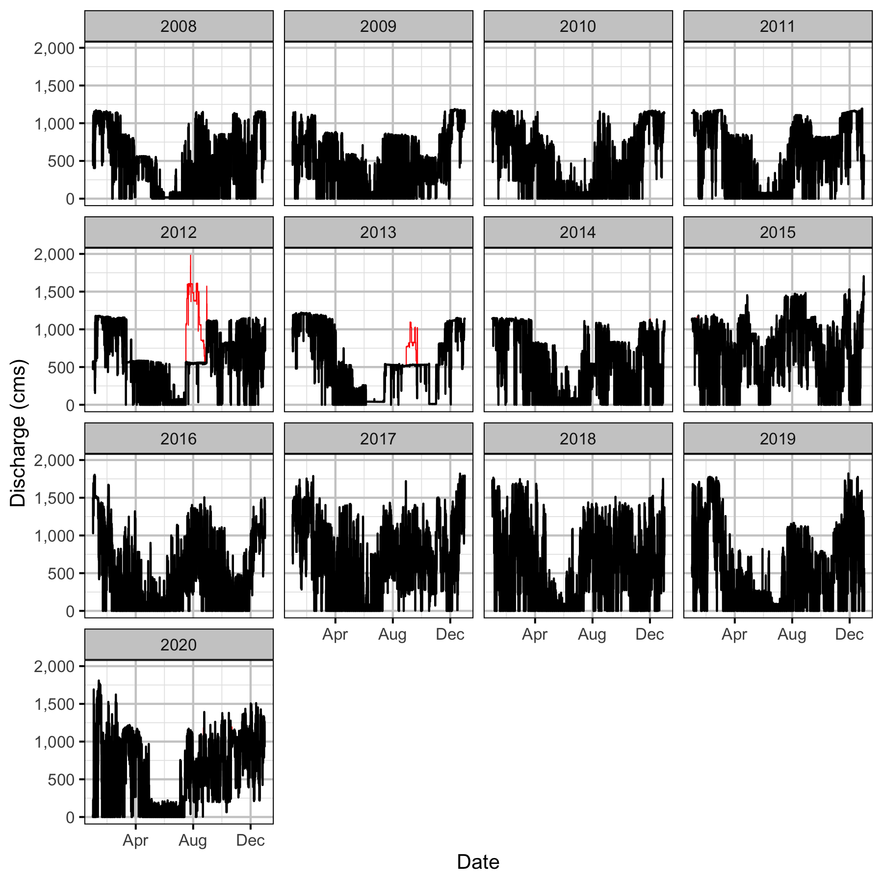
Figure 1. Hourly discharge from Mica Dam by turbines (black) and turbines plus spill (red).
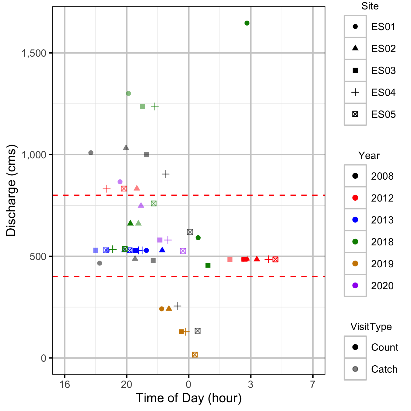
Figure 2. Mean discharge for the period three hours before and during each boat visit. The target discharge range is indicated by the horizontal red dashed lines.
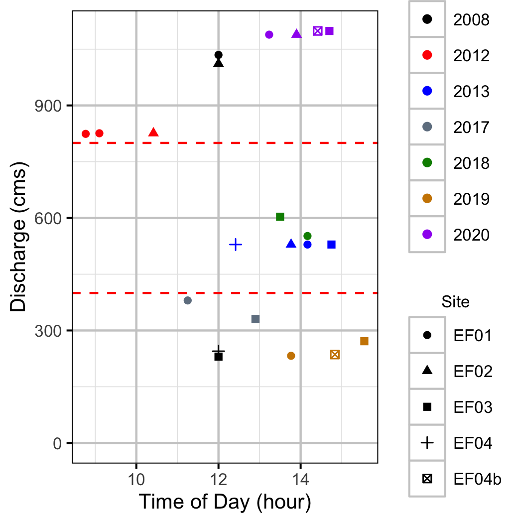
Figure 3. Mean discharge for the period three hours before and during each backpack visit. The target discharge range is indicated by the horizontal red dashed lines.
Condition
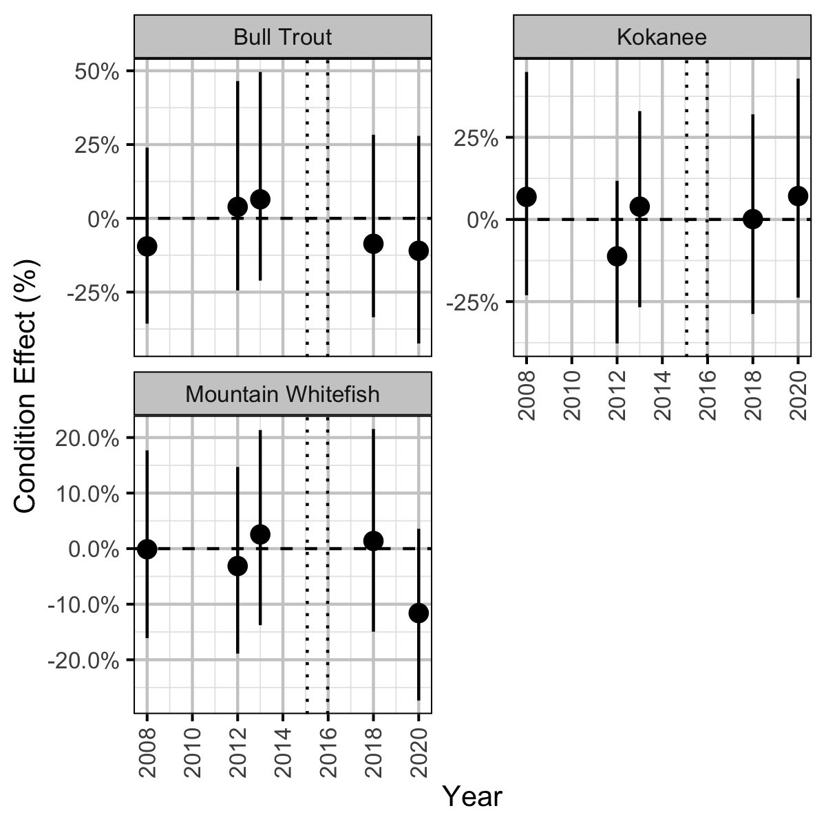
Figure 4. Estimated percent change in body condition by year relative to a typical year pre Mica 5 and 6 (with 95% CIs). The vertical dotted lines indicate the installation of Mica 5 and 6, respectively.
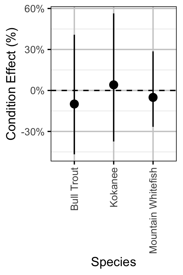
Figure 5. Estimated percent change in body condition associated with Mica 5 and 6 by species (with 95% CIs).
Relative Abundance
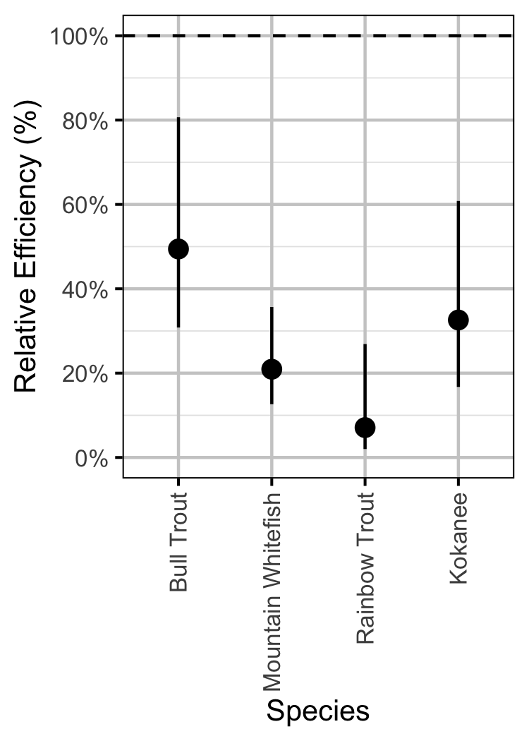
Figure 6. Relative efficiency of catching versus counting (with 95% CRIs).
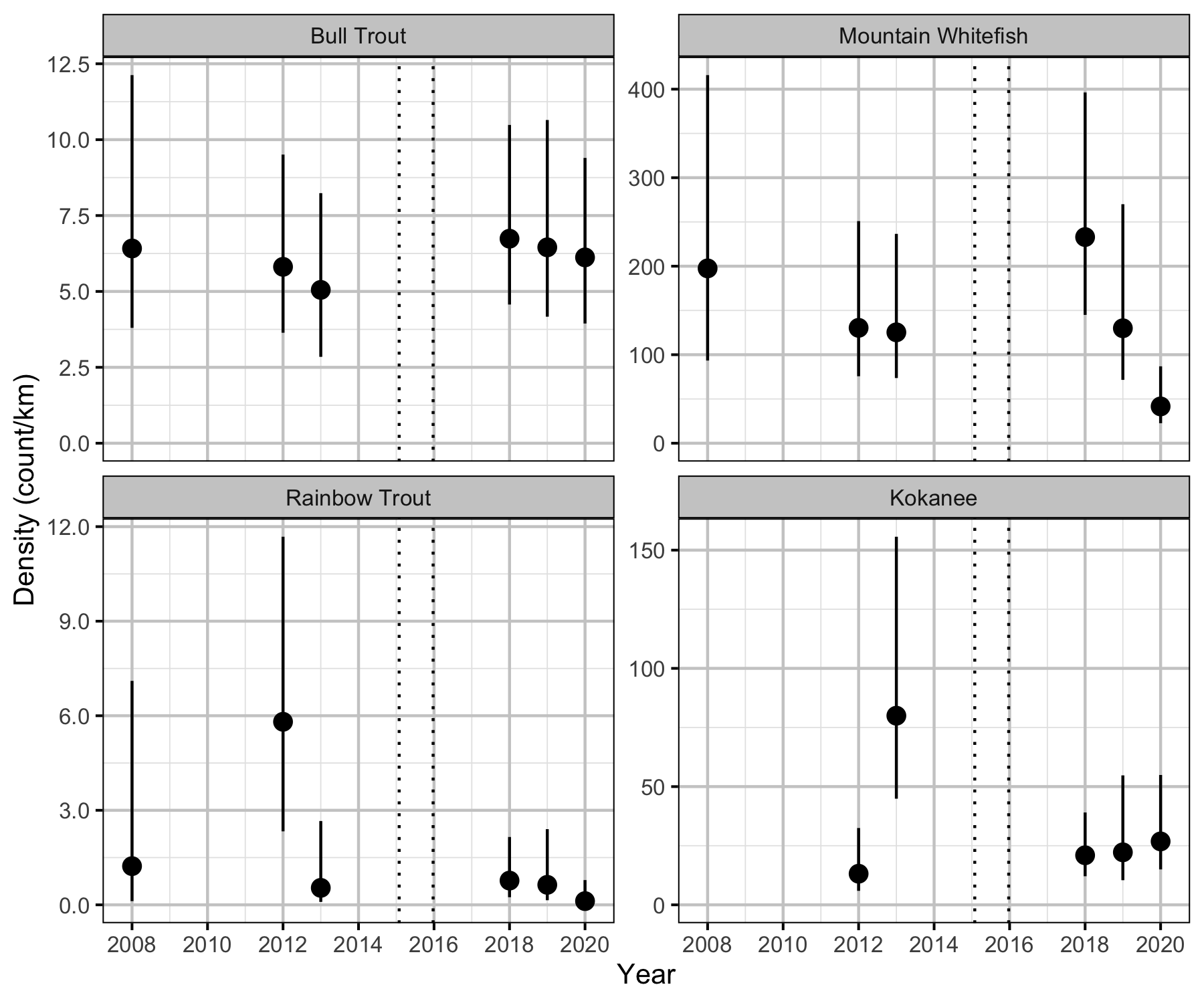
Figure 7. Estimated lineal count density (with 95% CRIs).
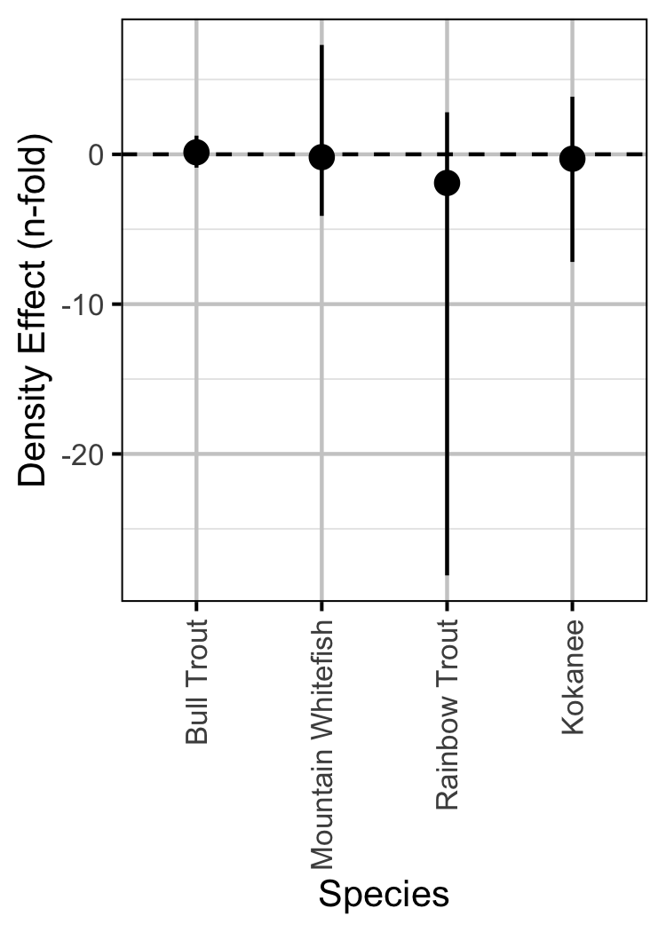
Figure 8. Estimated effect of Mica 5 and 6 on the lineal count density (with 95% CRIs).
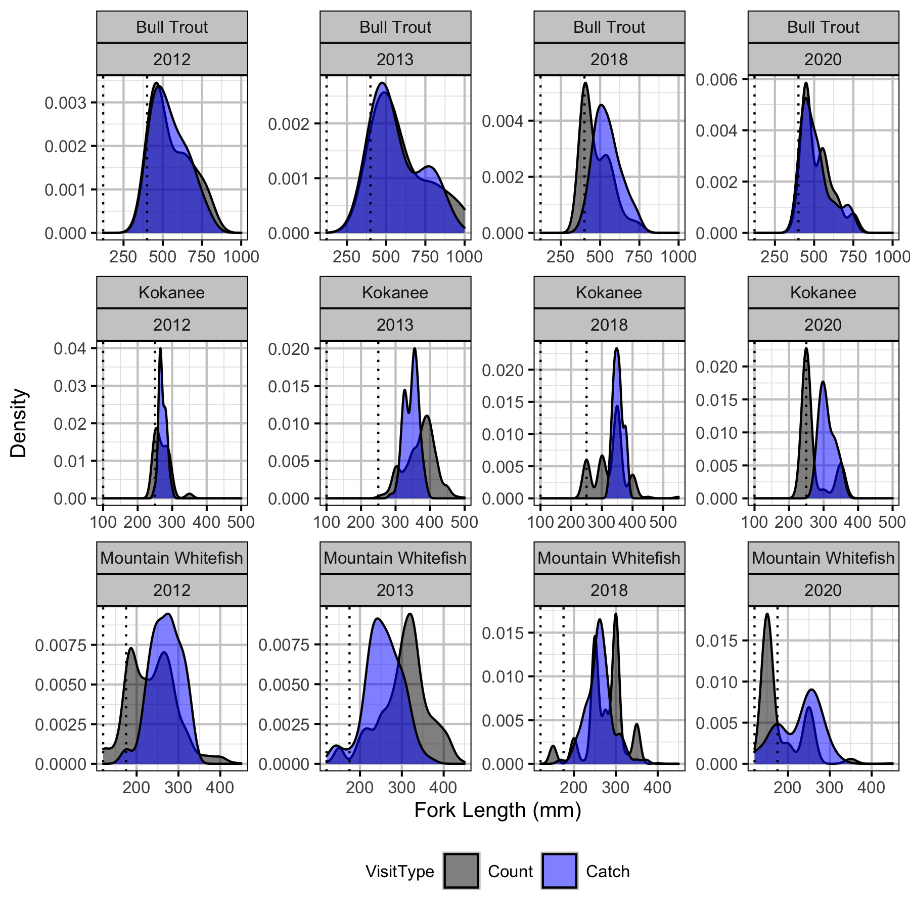
Figure 9. Length density by species and year for boat count versus boat catch for years with fry and juvenile cutoffs indicated by dotted vertical lines.
Bull Trout
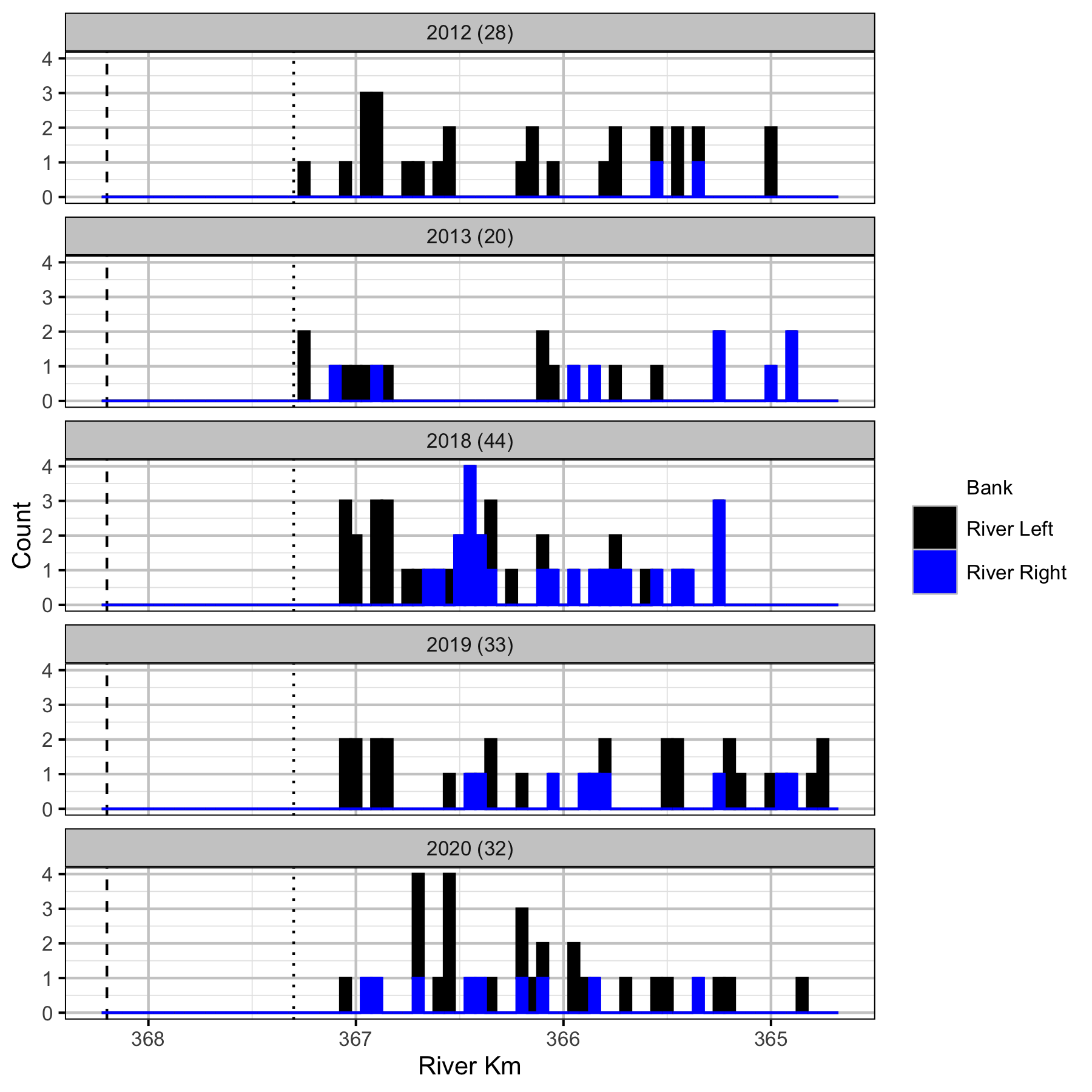
Figure 10. Boat counts by river km and bank for adult Bull Trout. Mica Dam is indicated by the vertical dashed line and the log boom by the vertical dotted line. The total count is in brackets after the year.
Mountain Whitefish
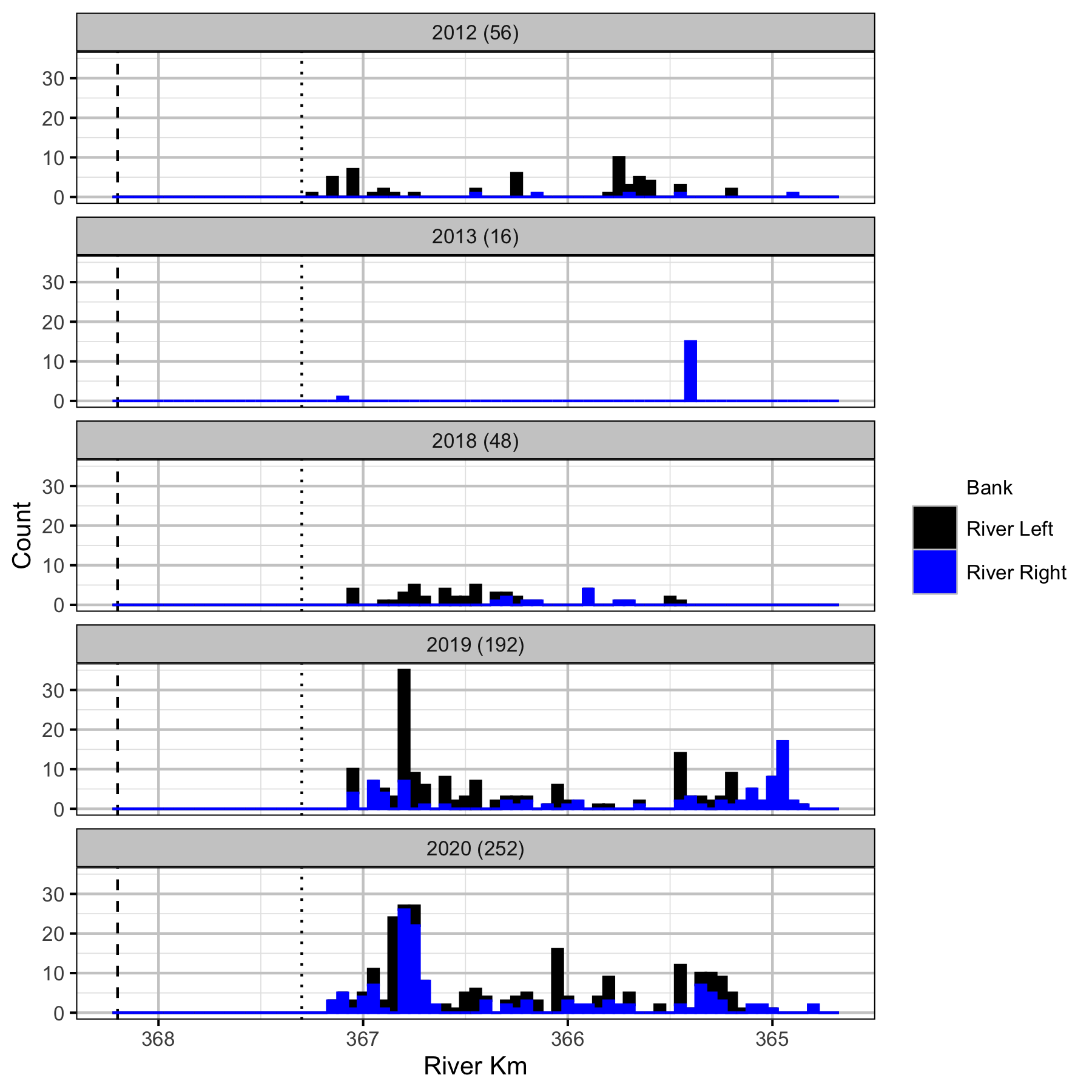
Figure 11. Boat counts by river km and bank for juvenile Mountain Whitefish. Mica Dam is indicated by the vertical dashed line and the log boom by the vertical dotted line. The total count is in brackets after the year.
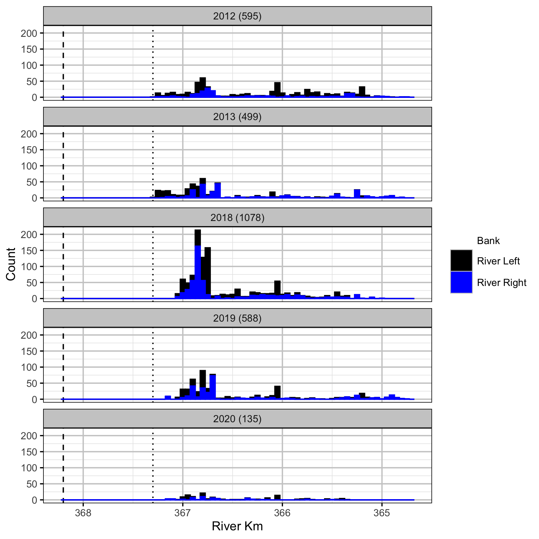
Figure 12. Boat counts by river km and bank for adult Mountain Whitefish. Mica Dam is indicated by the vertical dashed line and the log boom by the vertical dotted line. The total count is in brackets after the year.
Rainbow Trout
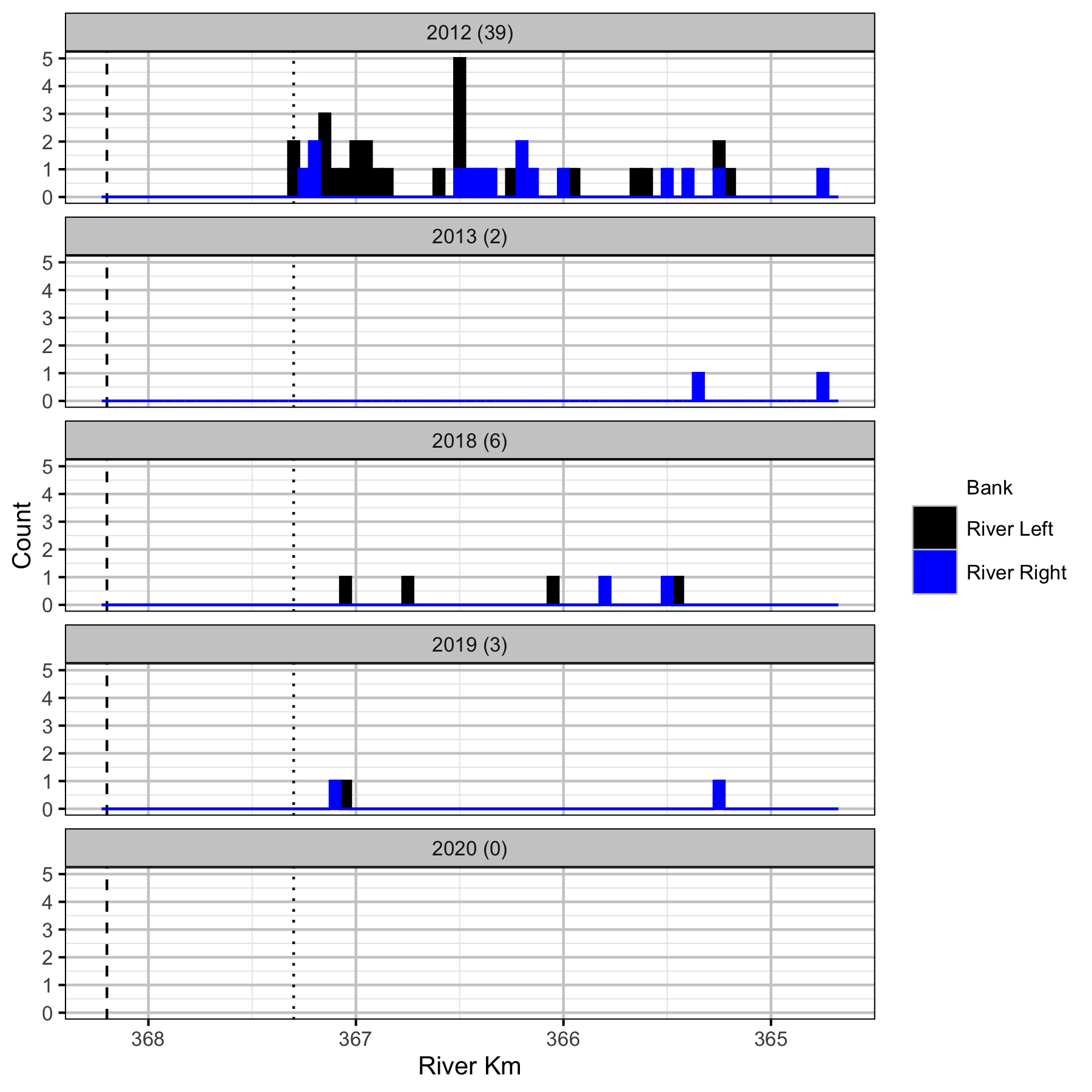
Figure 13. Boat counts by river km and bank for adult Rainbow Trout. Mica Dam is indicated by the vertical dashed line and the log boom by the vertical dotted line. The total count is in brackets after the year.
Kokanee
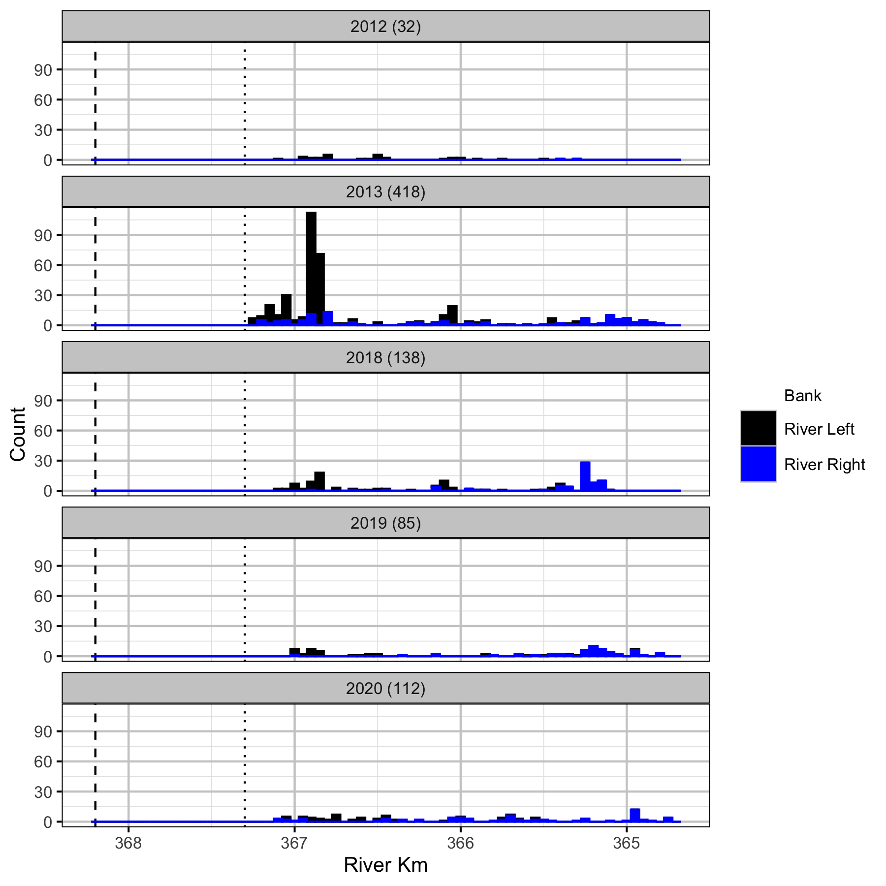
Figure 14. Boat counts by river km and bank for adult Kokanee. Mica Dam is indicated by the vertical dashed line and the log boom by the vertical dotted line. The total count is in brackets after the year.
Backpack Electrofishing
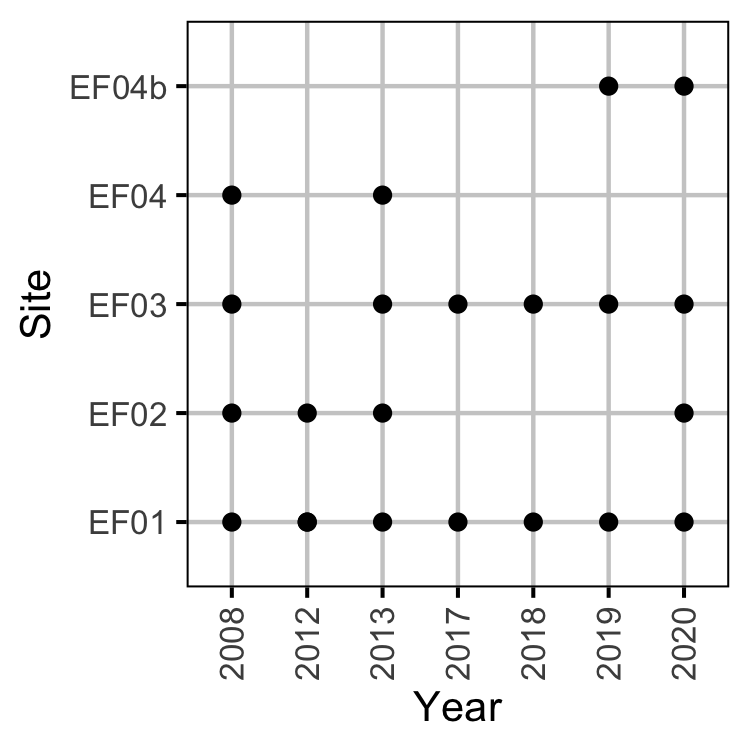
Figure 15. Backpack electrofishing site visits by year.
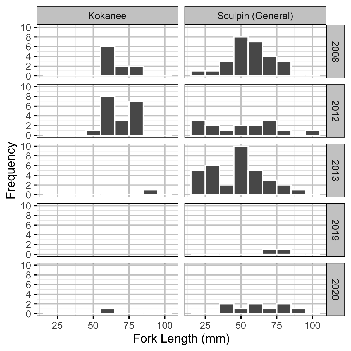
Figure 16. Length-frequency histogram of fish caught by backpack electrofishing by species and year. The plot excludes kokanee greater than 200 mm and one mountain whitefish that was caught in 2019.
Temperature
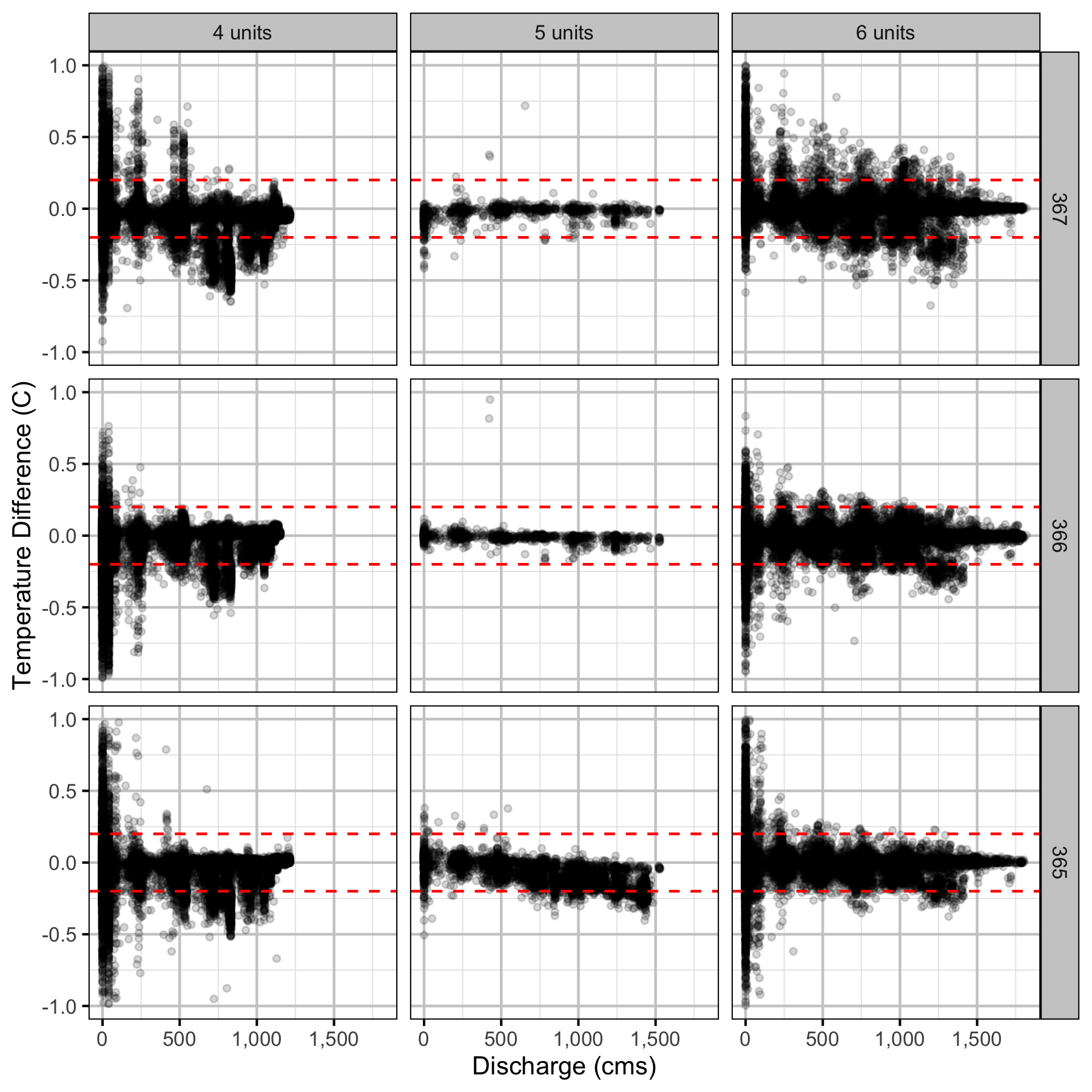
Figure 17. The hourly water temperature difference between the right versus left bank by discharge, regime and river km for absolute differences less than or equal to 1 C. The redd dashed lines indicate the accuracy of a temperature logger.
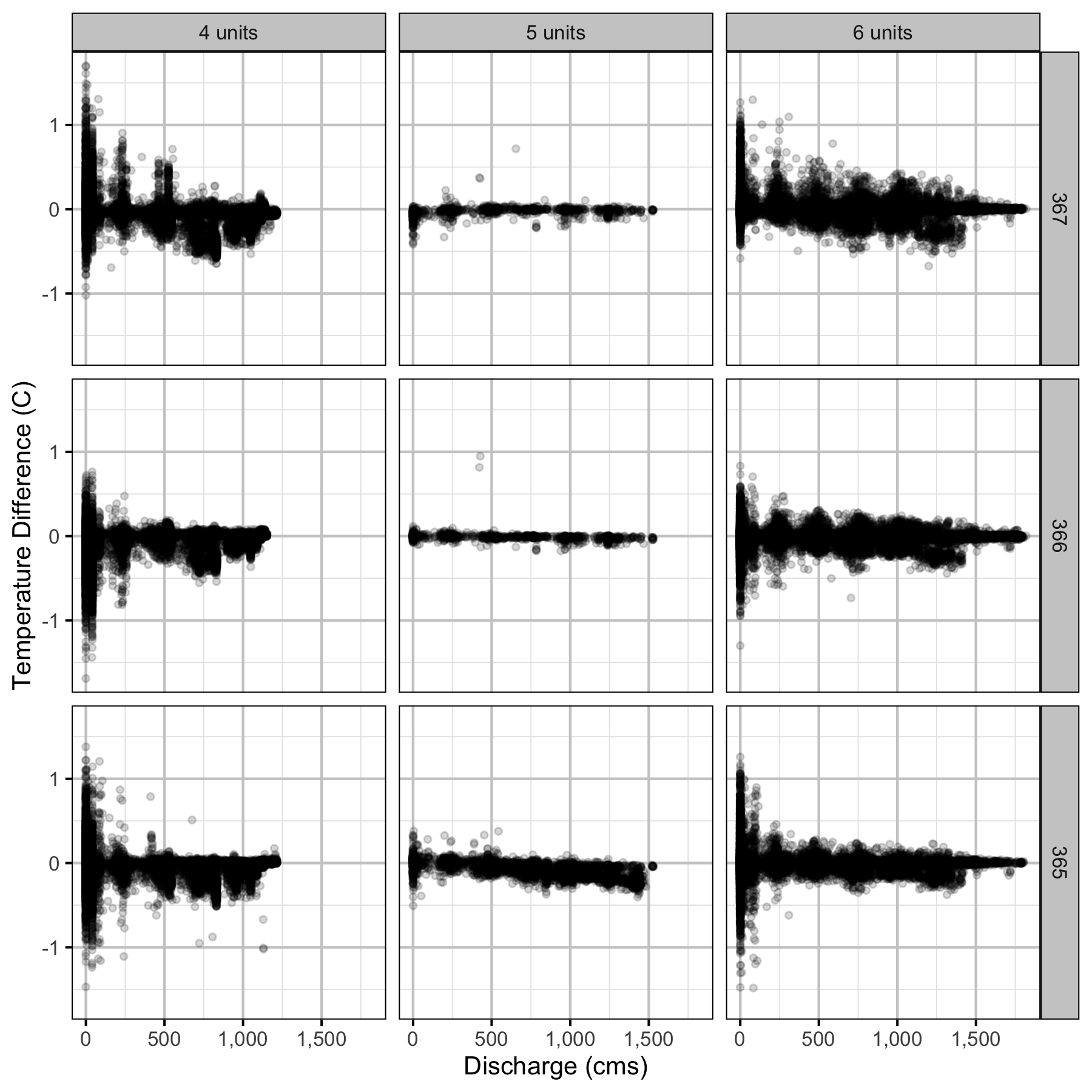
Figure 18. The hourly water temperature difference between the right versus left bank by discharge, regime and river km for all differences.
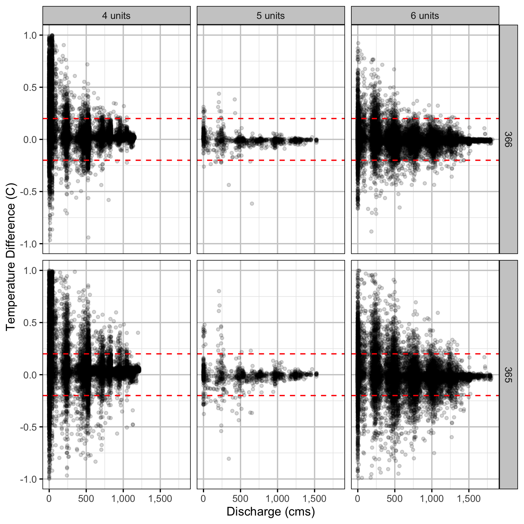
Figure 19. The hourly water temperature difference compared to 367 river km by discharge, regime and river km for absolute differences less than or equal to 1.0 C. The redd dashed lines indicate the accuracy of a temperature logger.
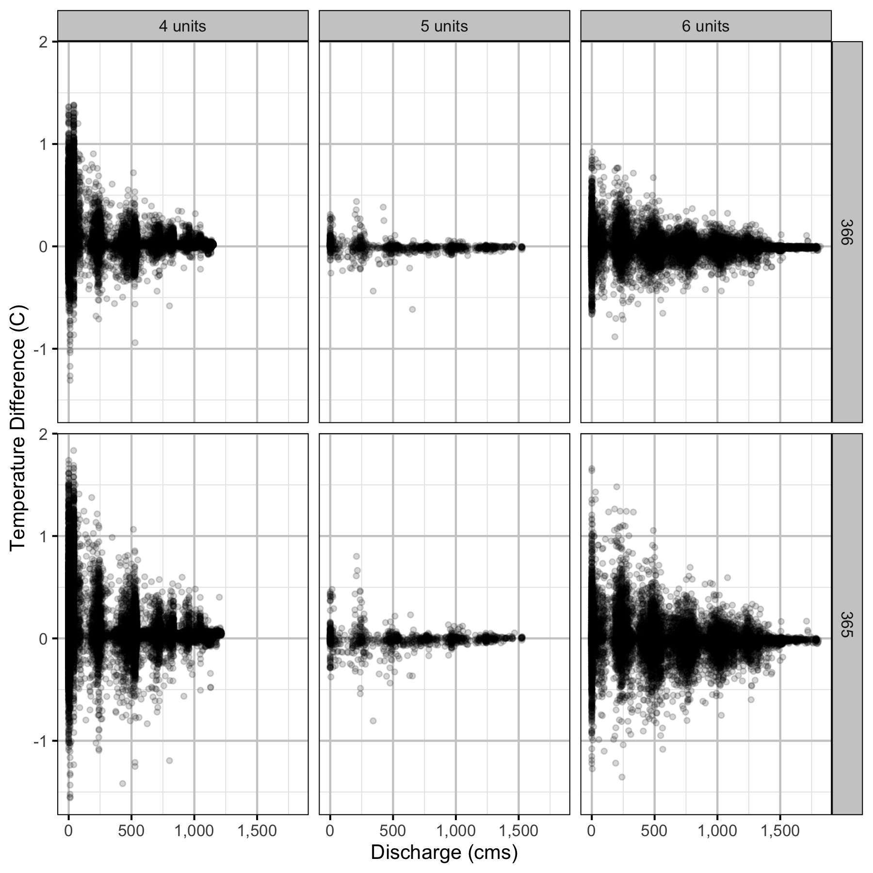
Figure 20. The hourly water temperature difference compared to 367 river km by discharge, regime and river km for all differences.
Tailrace
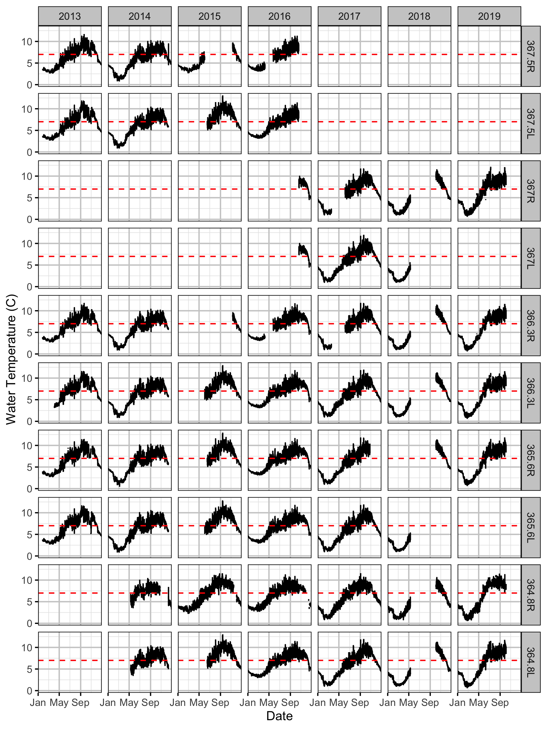
Figure 21. Hourly water temperature in Mica Dam tailrace by date, year and site.
Forebay
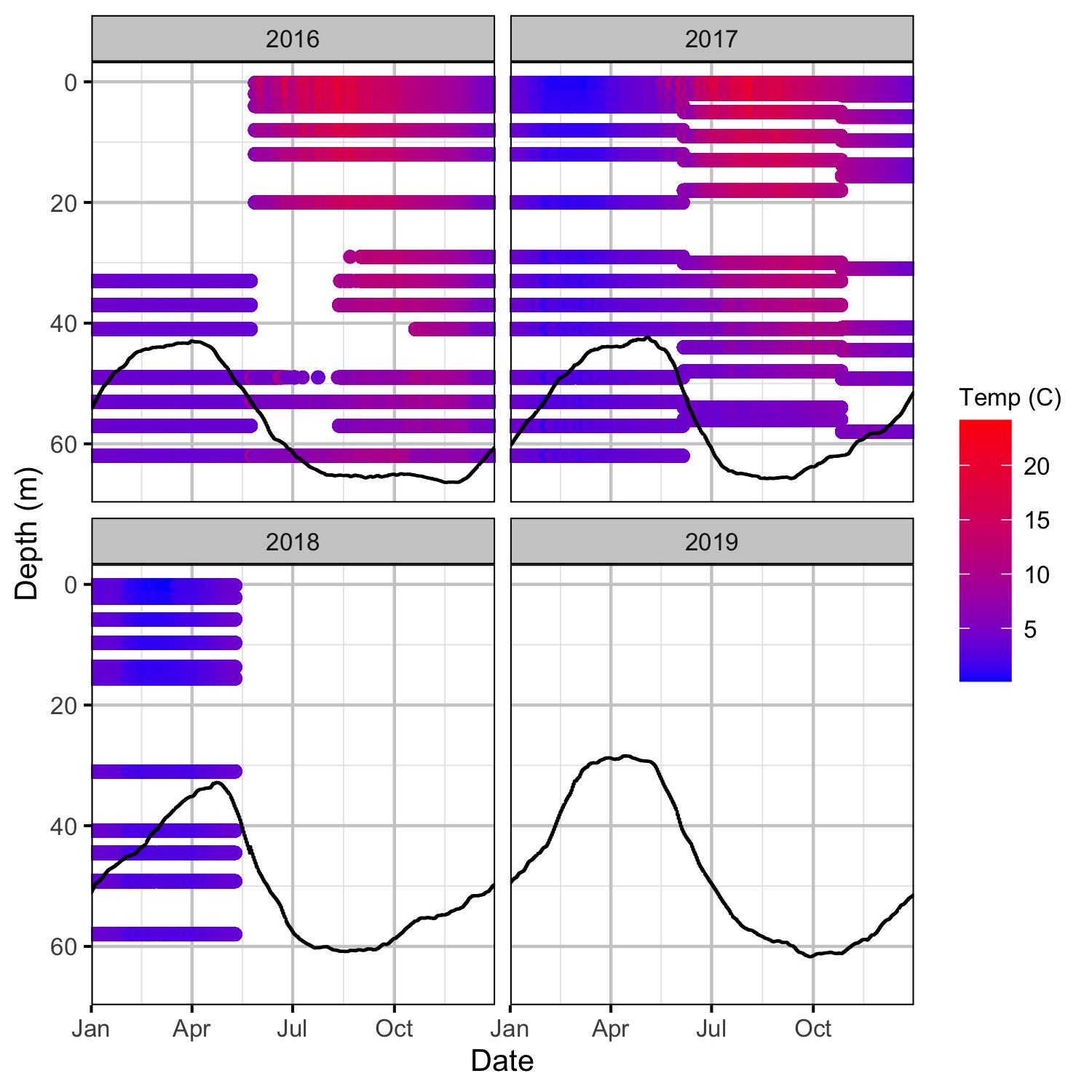
Figure 22. Hourly water temperature in Mica Dam forebay by date, depth and year.
Forebay and Tailrace
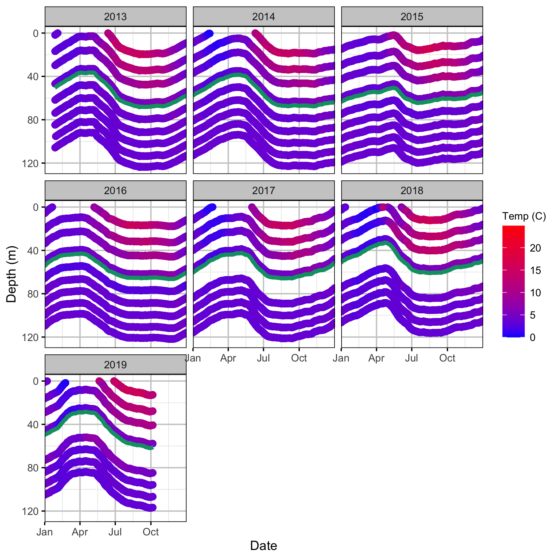
Figure 23. The dam thermistor water temperatures by date, depth and year. The green line indicates the turbine intake depth of 686.41 masl.
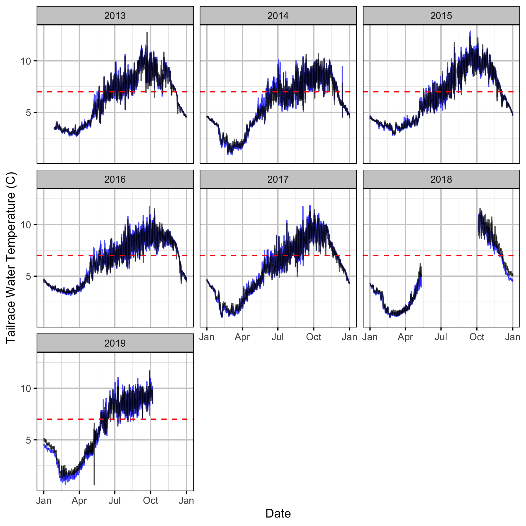
Figure 24. The actual (in red) and estimated (in black) hourly tailrace water temperature by date and year.
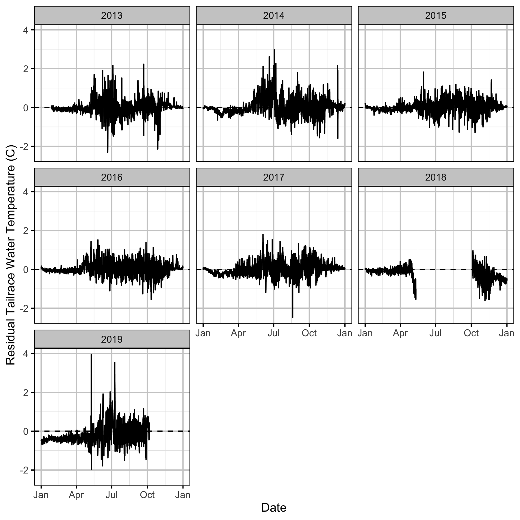
Figure 25. The raw residual hourly tailrace water temperature by date and year.
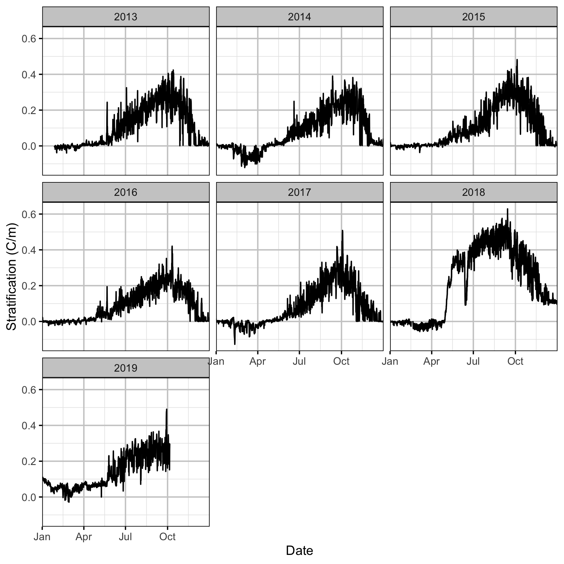
Figure 26. The hourly water temperature stratification between the thermistor at 707 masl and the thermistor at 690 masl by date and year.
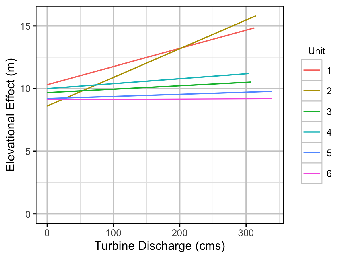
Figure 27. The estimated elevational effect relative to the thermistor at 690 masl by the turbine discharge and unit.
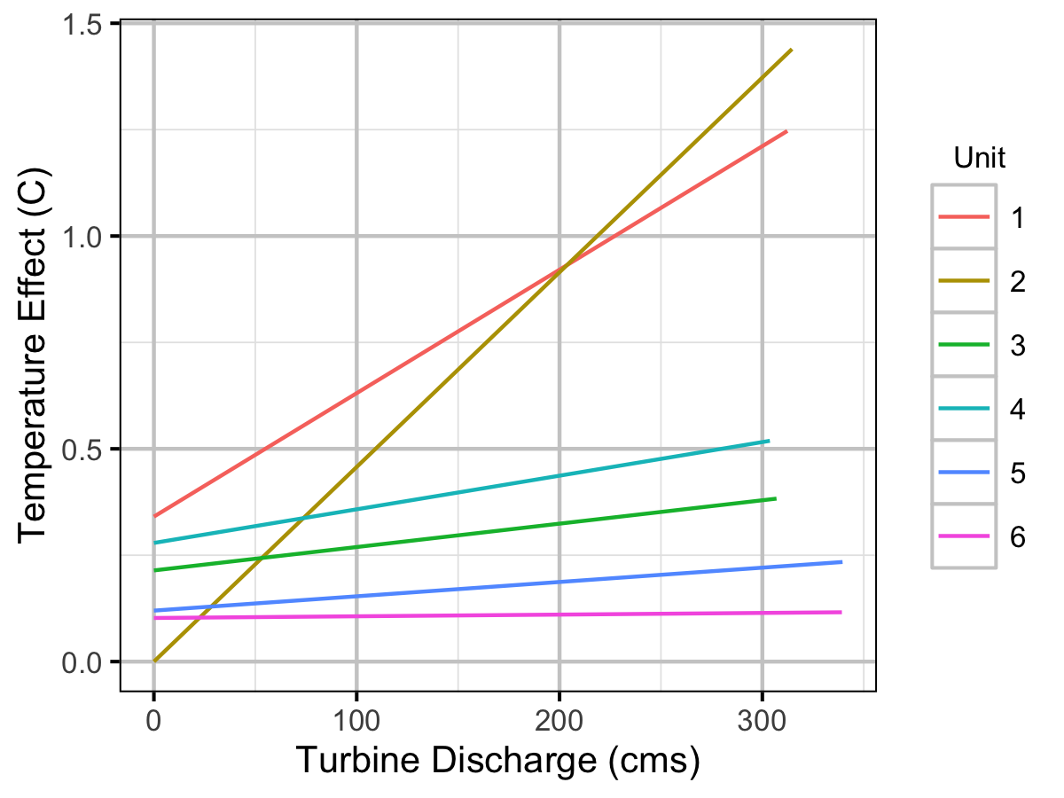
Figure 28. The estimated temperature effect relative to no discharge by the turbine discharge and unit.
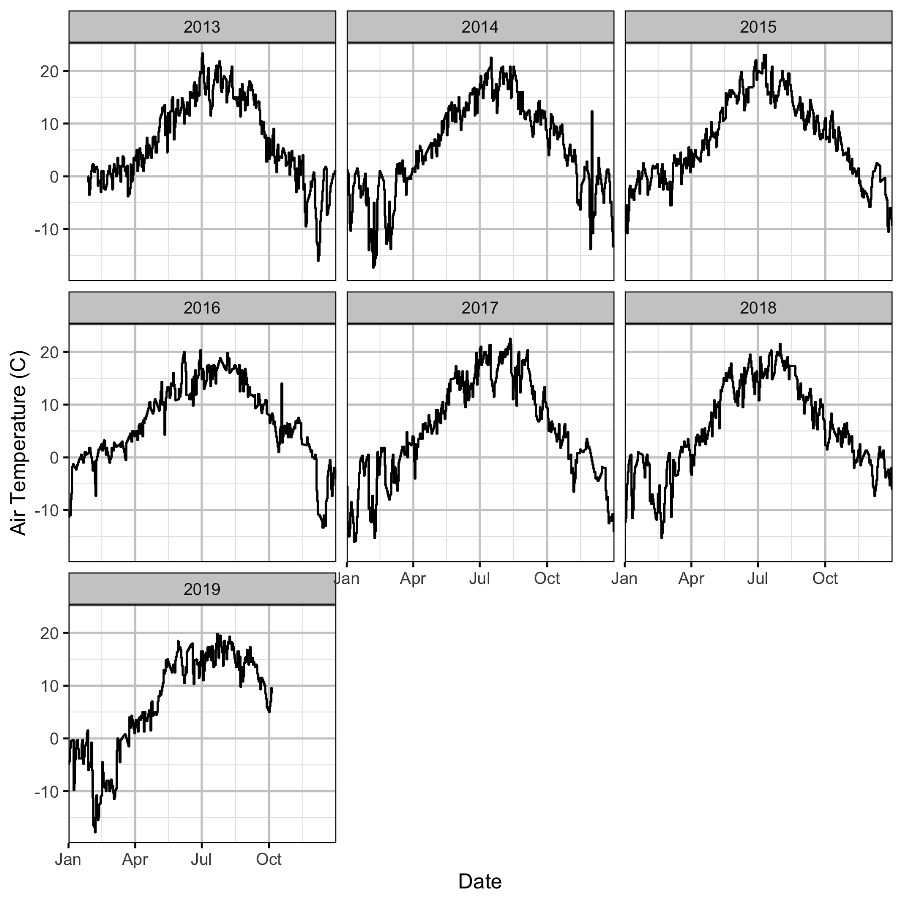
Figure 29. The mean daily air temperature at the Mica weather station by date and year.
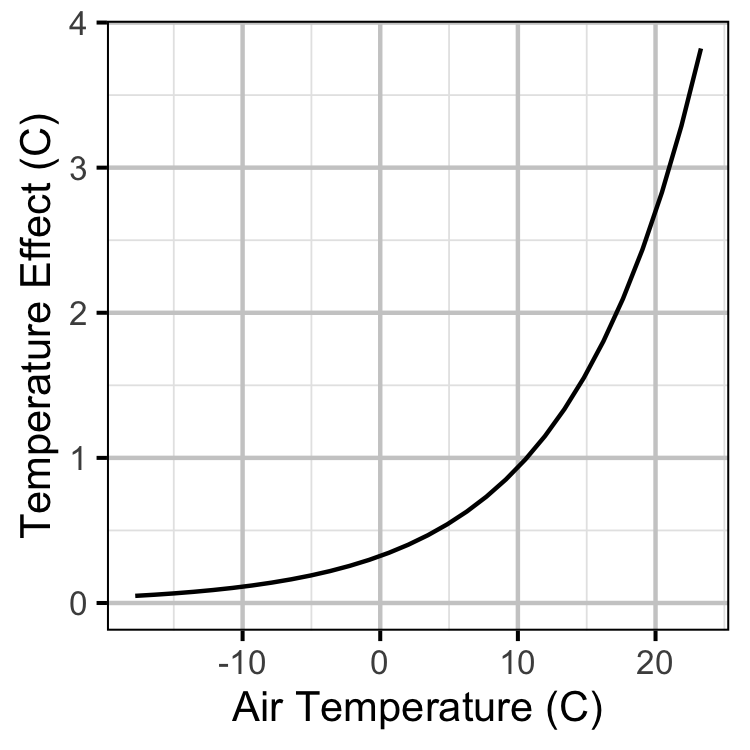
Figure 30. The estimated effect of the difference between the mean daily air temperature and the temperature at the thermistor at 690 masl on the discharge temperature.
Maps
Sites
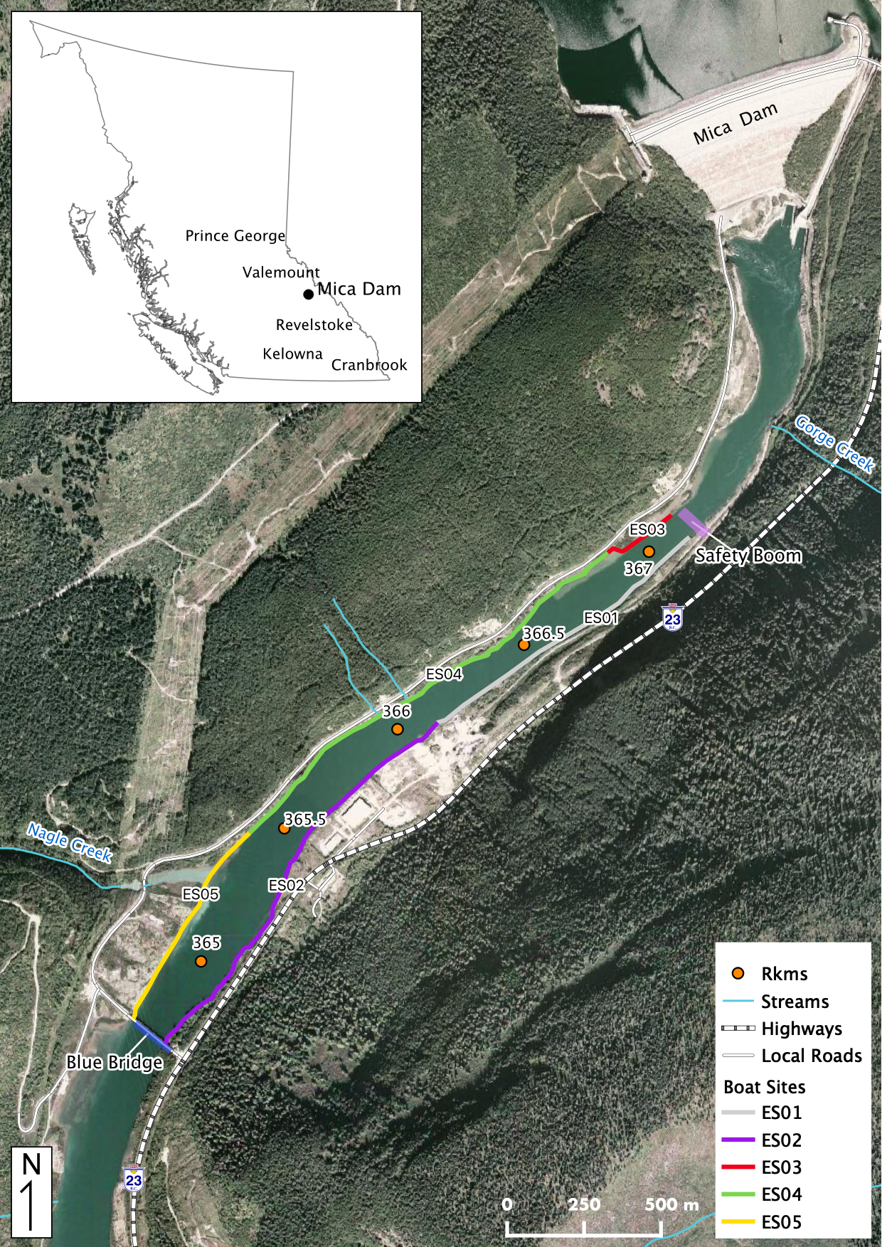
Figure 31. Overview map of Boat Electrofishing (ES) sites.
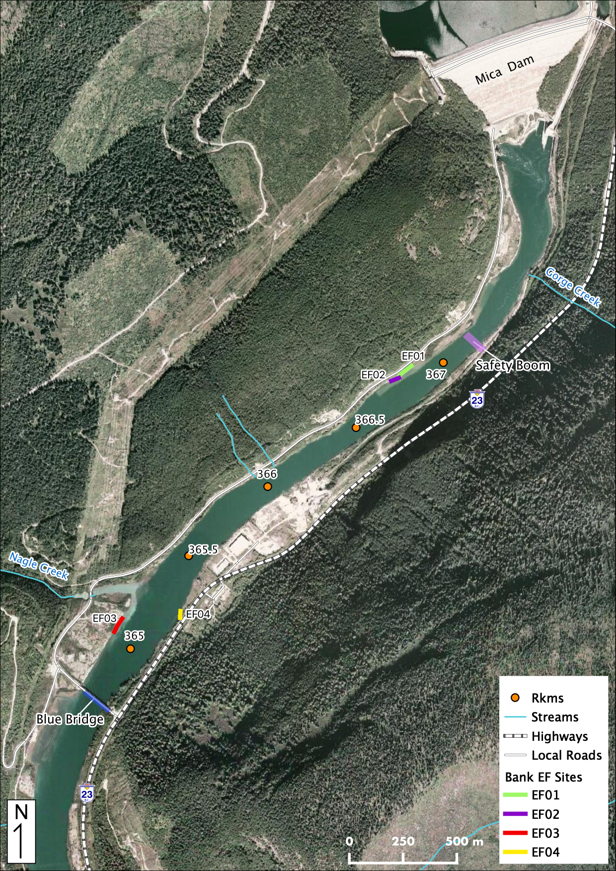
Figure 32. Overview map of Backpack Electrofishing (EF) sites.
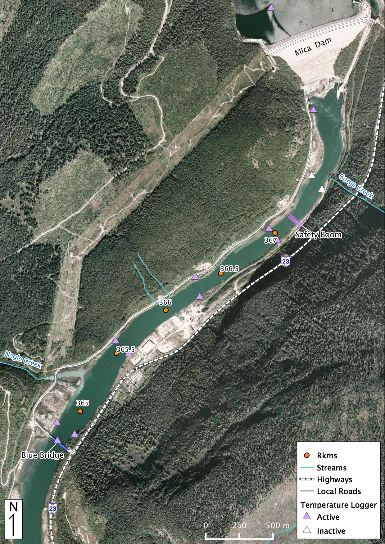
Figure 33. Overview map of Tidbit temperature logger deployment locations for 2019.
Relative Distributions
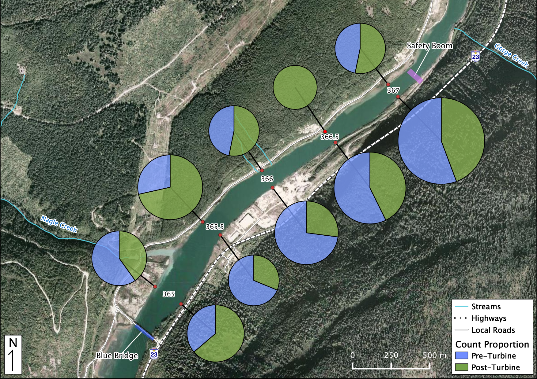
Figure 34. Relative Distribution of Adult Bull Trout. The sections in each piechart indicate the relative proportion of counts Pre vs Post-Turbine within that location while the size of each piechart indicates the distribution among locations.
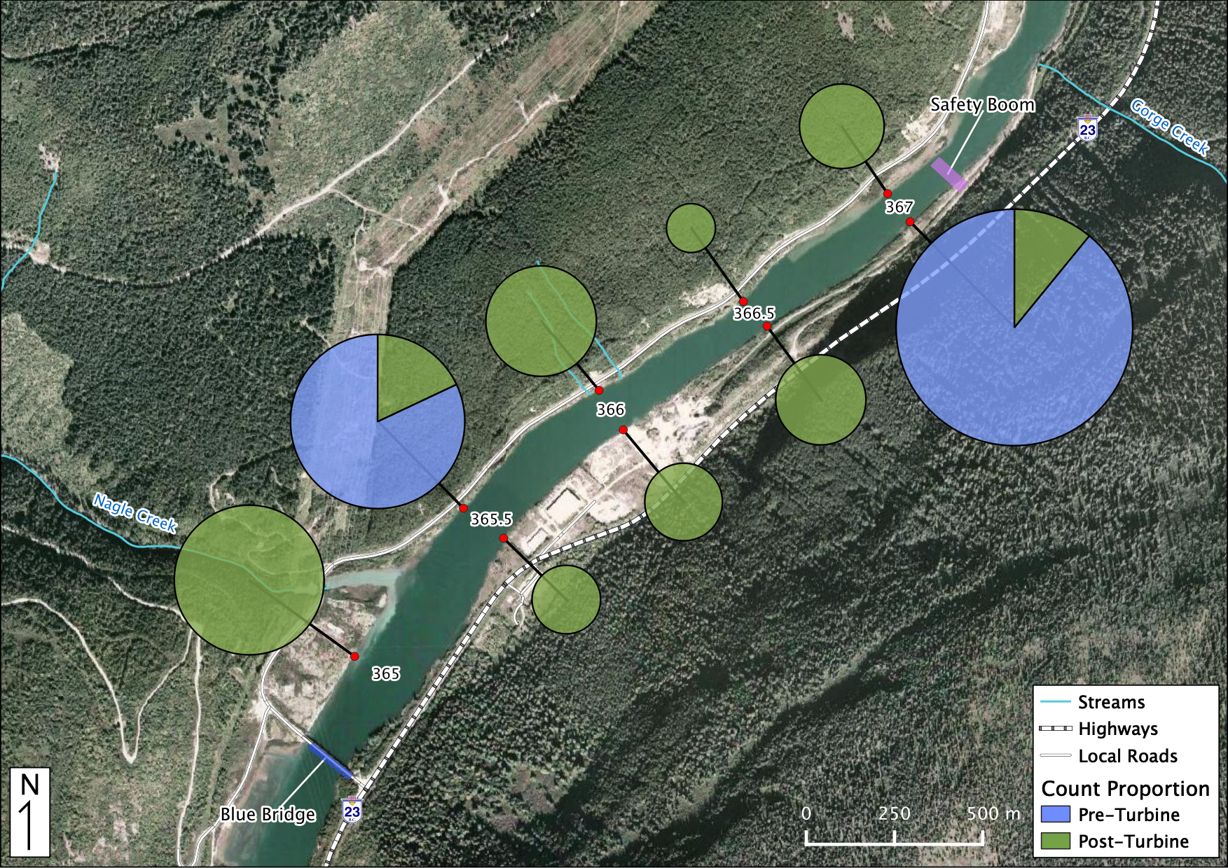
Figure 35. Relative Distribution of Juvenile Bull Trout. The sections in each piechart indicate the relative proportion of counts Pre vs Post-Turbine within that location while the size of each piechart indicates the distribution among locations.
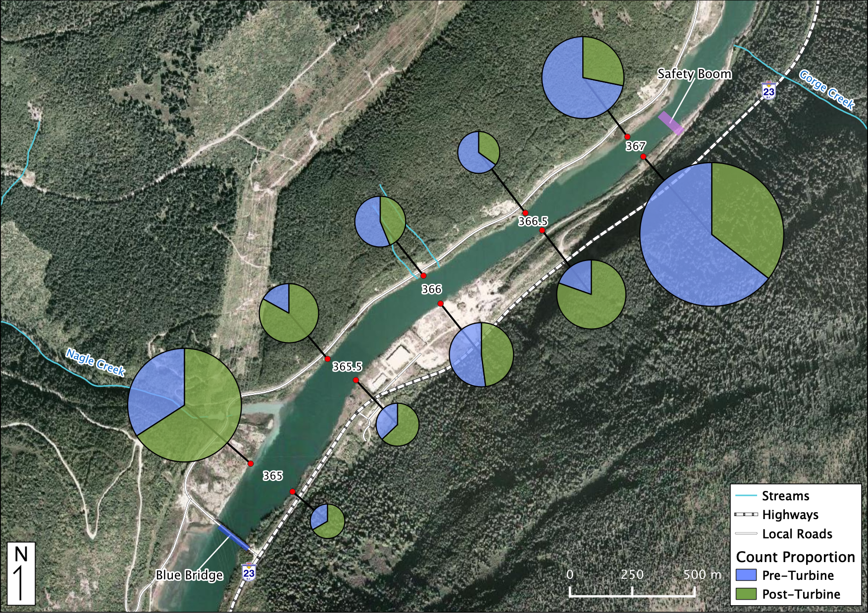
Figure 36. Relative Distribution of Adult Kokanee. The sections in each piechart indicate the relative proportion of counts Pre vs Post-Turbine within that location while the size of each piechart indicates the distribution among locations.
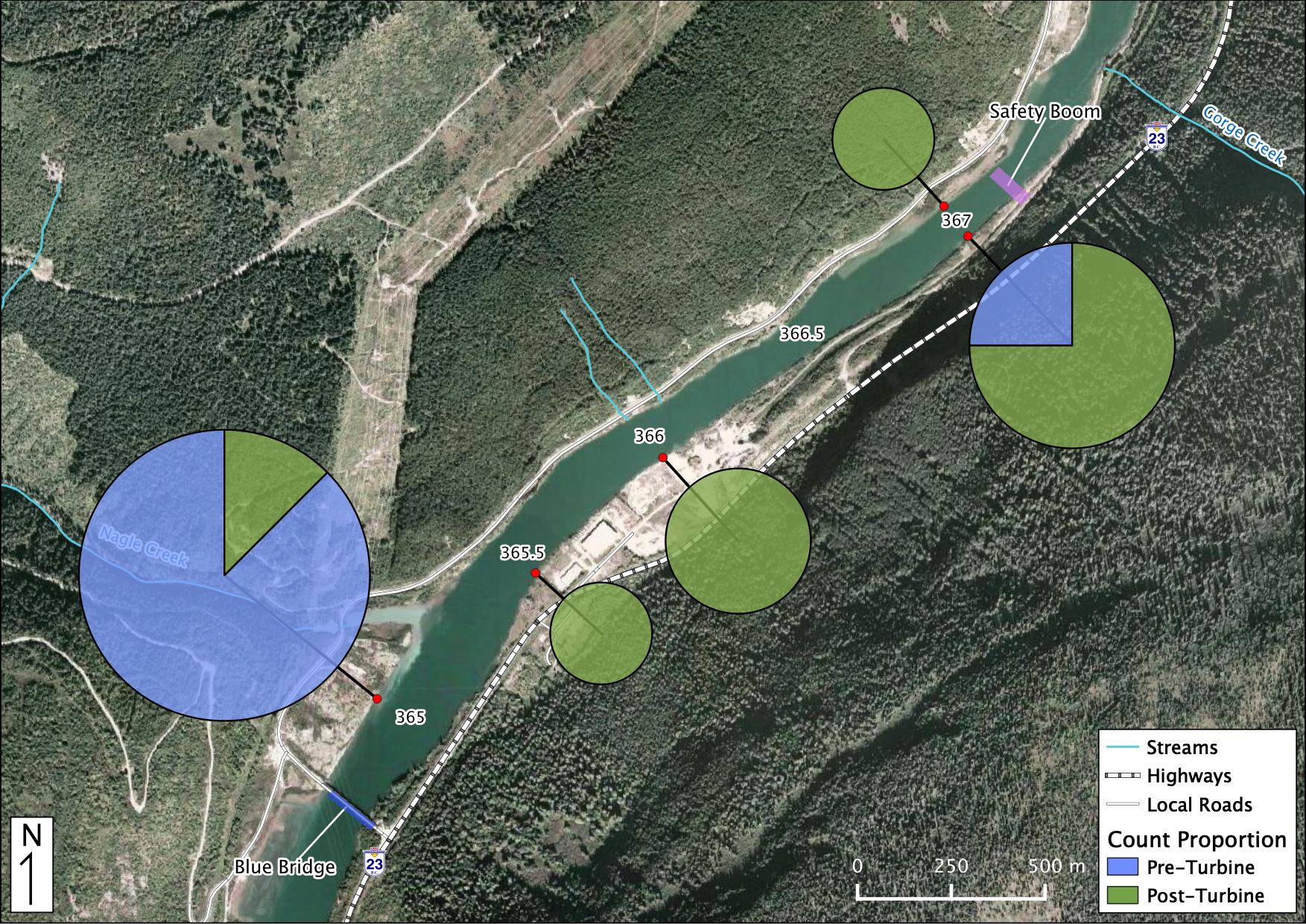
Figure 37. Relative Distribution of Fry Kokanee. The sections in each piechart indicate the relative proportion of counts Pre vs Post-Turbine within that location while the size of each piechart indicates the distribution among locations.
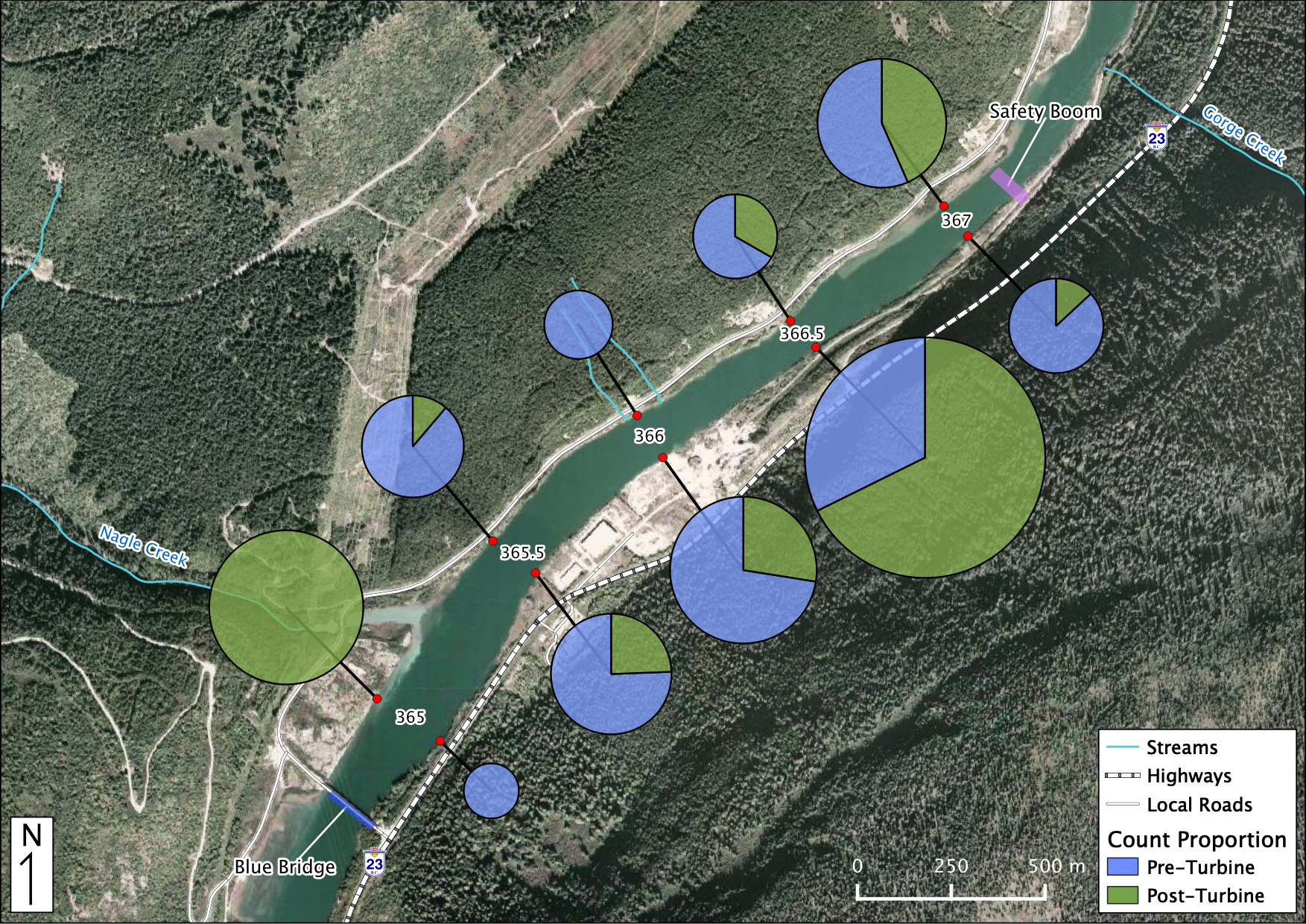
Figure 38. Relative Distribution of Juvenile Kokanee. The sections in each piechart indicate the relative proportion of counts Pre vs Post-Turbine within that location while the size of each piechart indicates the distribution among locations.
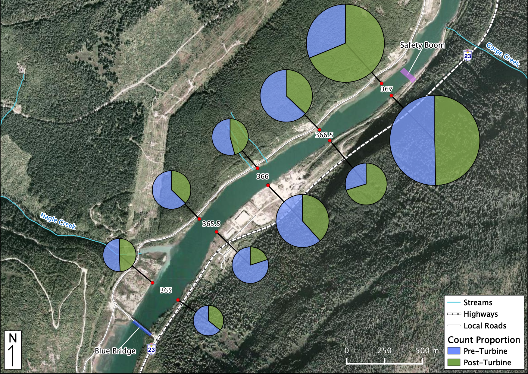
Figure 39. Relative Distribution of Adult Mountain Whitefish. The sections in each piechart indicate the relative proportion of counts Pre vs Post-Turbine within that location while the size of each piechart indicates the distribution among locations.
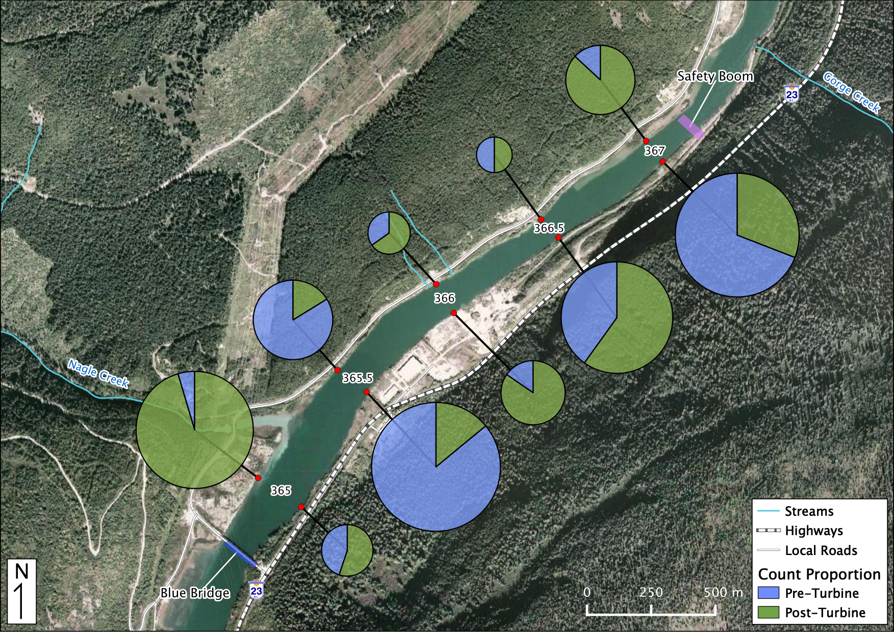
Figure 40. Relative Distribution of Juvenile Mountain Whitefish. The sections in each piechart indicate the relative proportion of counts Pre vs Post-Turbine within that location while the size of each piechart indicates the distribution among locations.
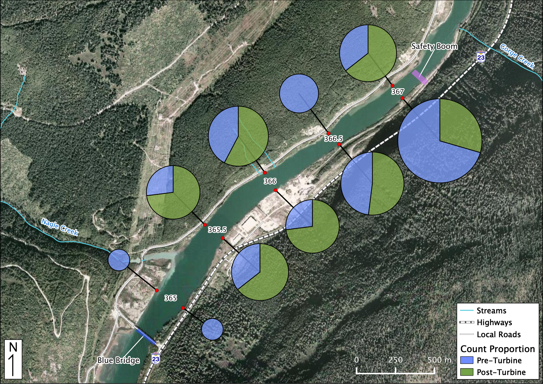
Figure 41. Relative Distribution of Adult Rainbow Trout. The sections in each piechart indicate the relative proportion of counts Pre vs Post-Turbine within that location while the size of each piechart indicates the distribution among locations.
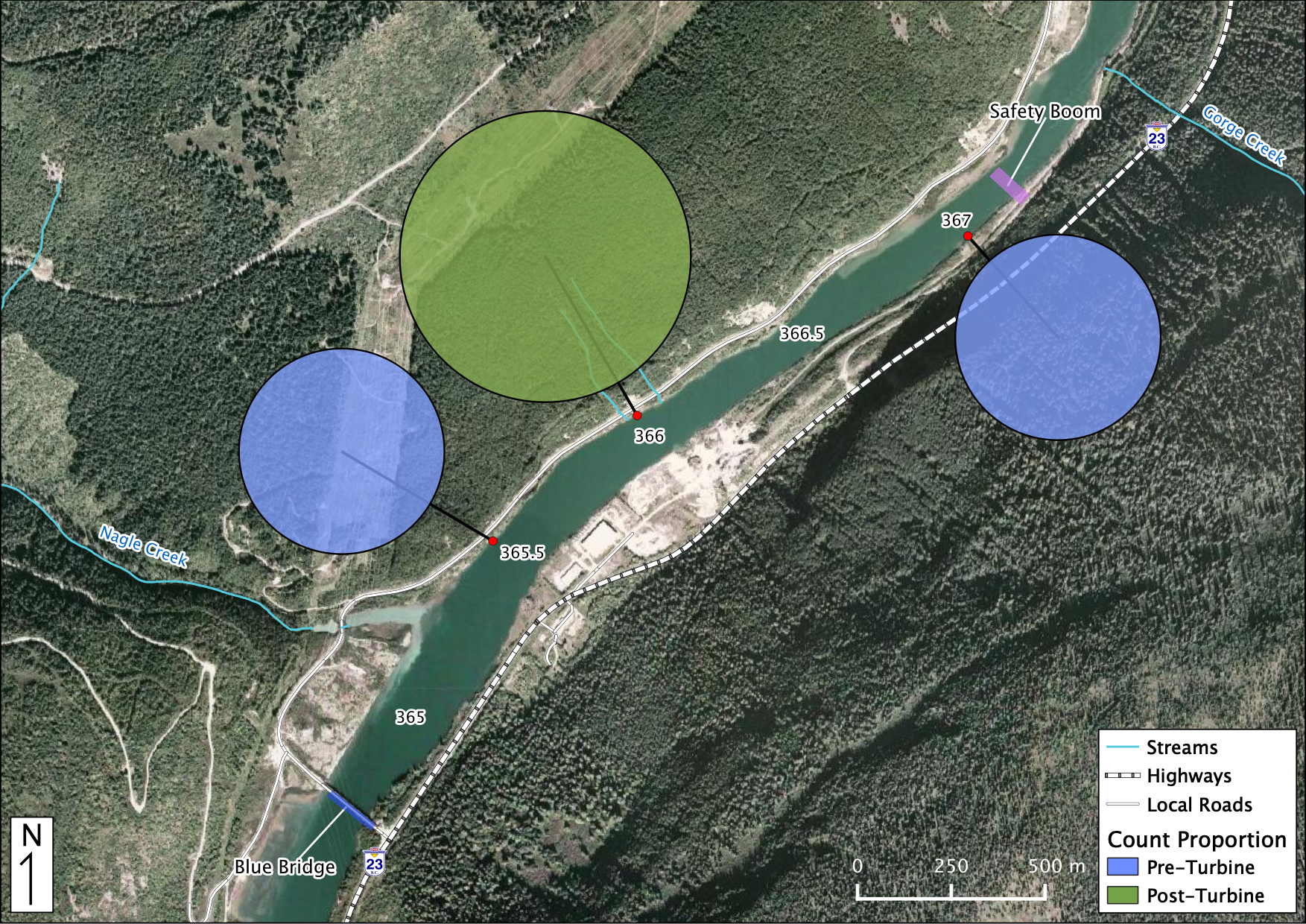
Figure 42. Relative Distribution of Juvenile Rainbow Trout. The sections in each piechart indicate the relative proportion of counts Pre vs Post-Turbine within that location while the size of each piechart indicates the distribution among locations.
Boat Counts
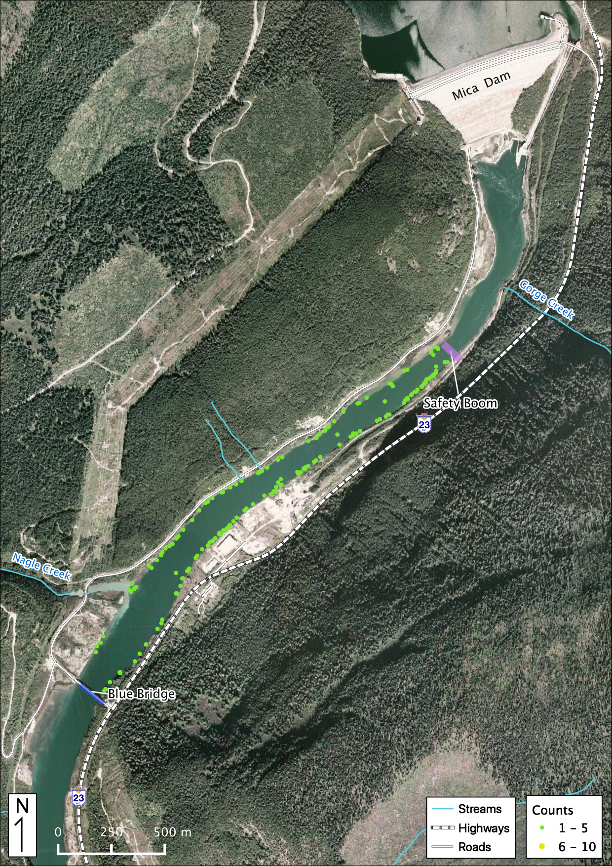
Figure 43. All Bull Trout observations in the study area below Mica Dam.
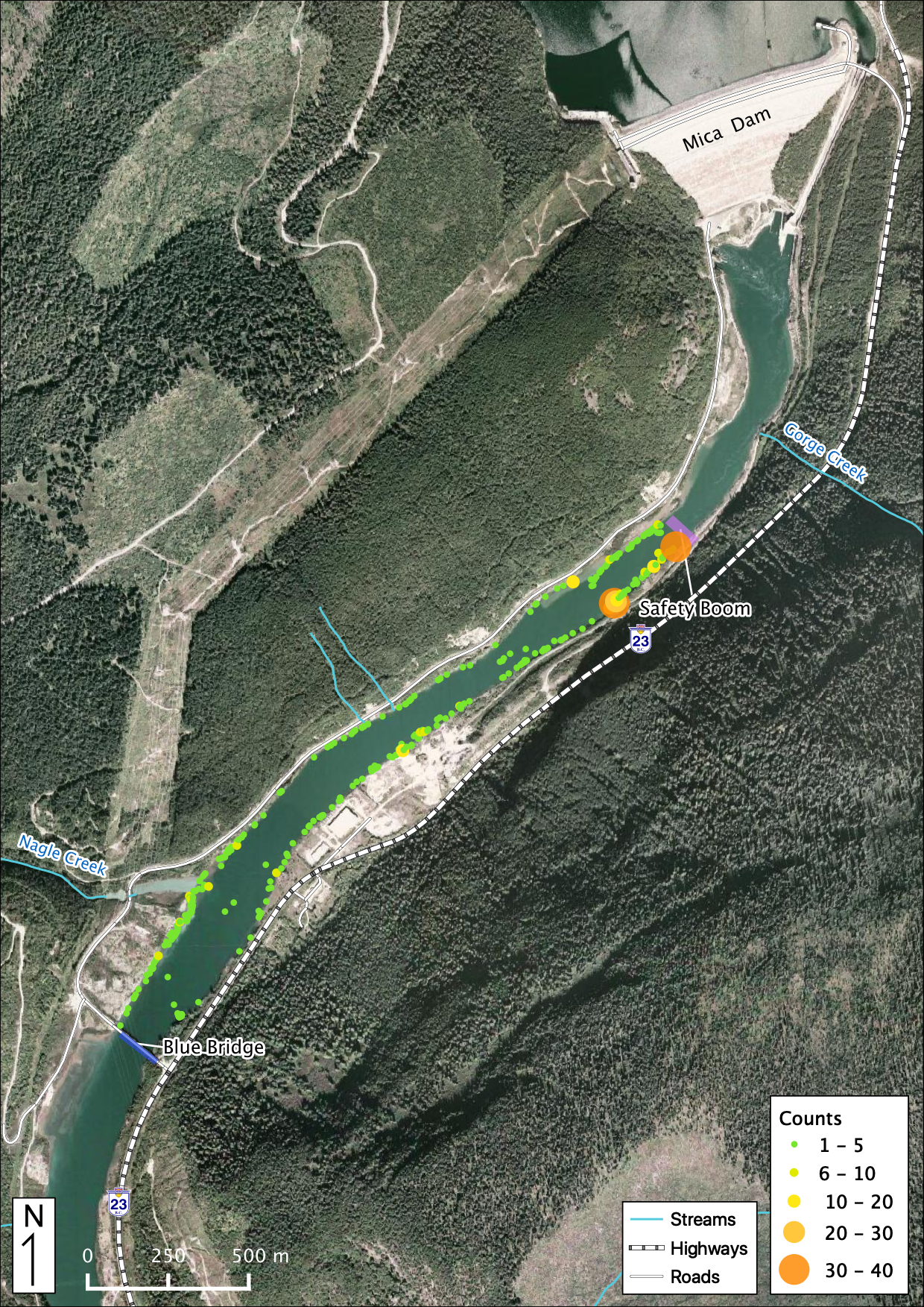
Figure 44. All Kokanee observations in the study area below Mica Dam.
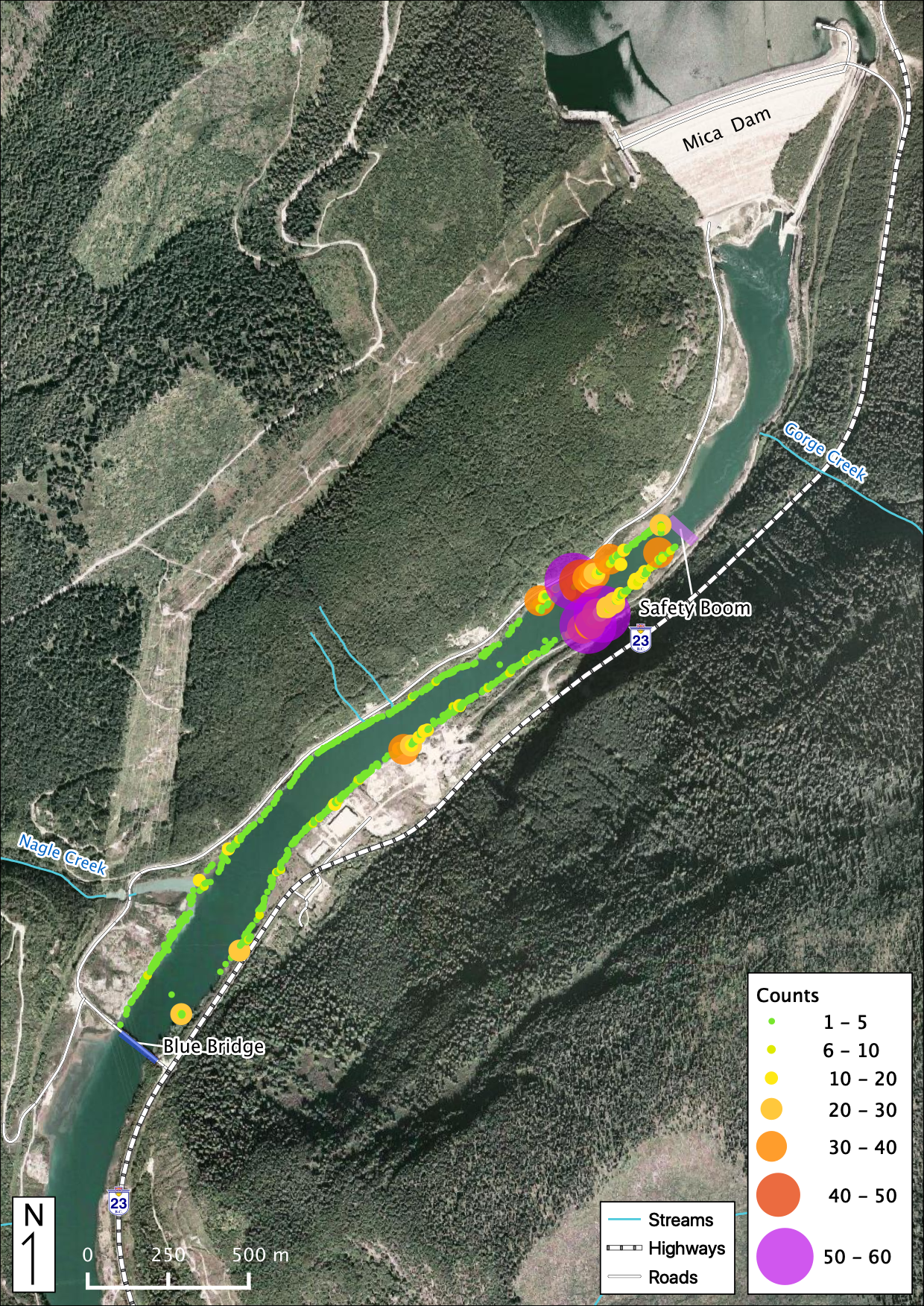
Figure 45. All Mountain Whitefish observations in the study area below Mica Dam.
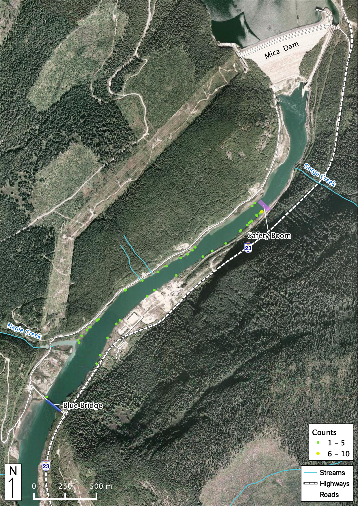
Figure 46. All Rainbow Trout observations in the study area below Mica Dam.

Figure 47. Adult Bull Trout observations in the study area below Mica Dam.
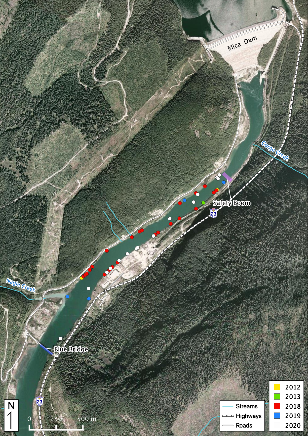
Figure 48. Juvenile Bull Trout observations in the study area below Mica Dam.
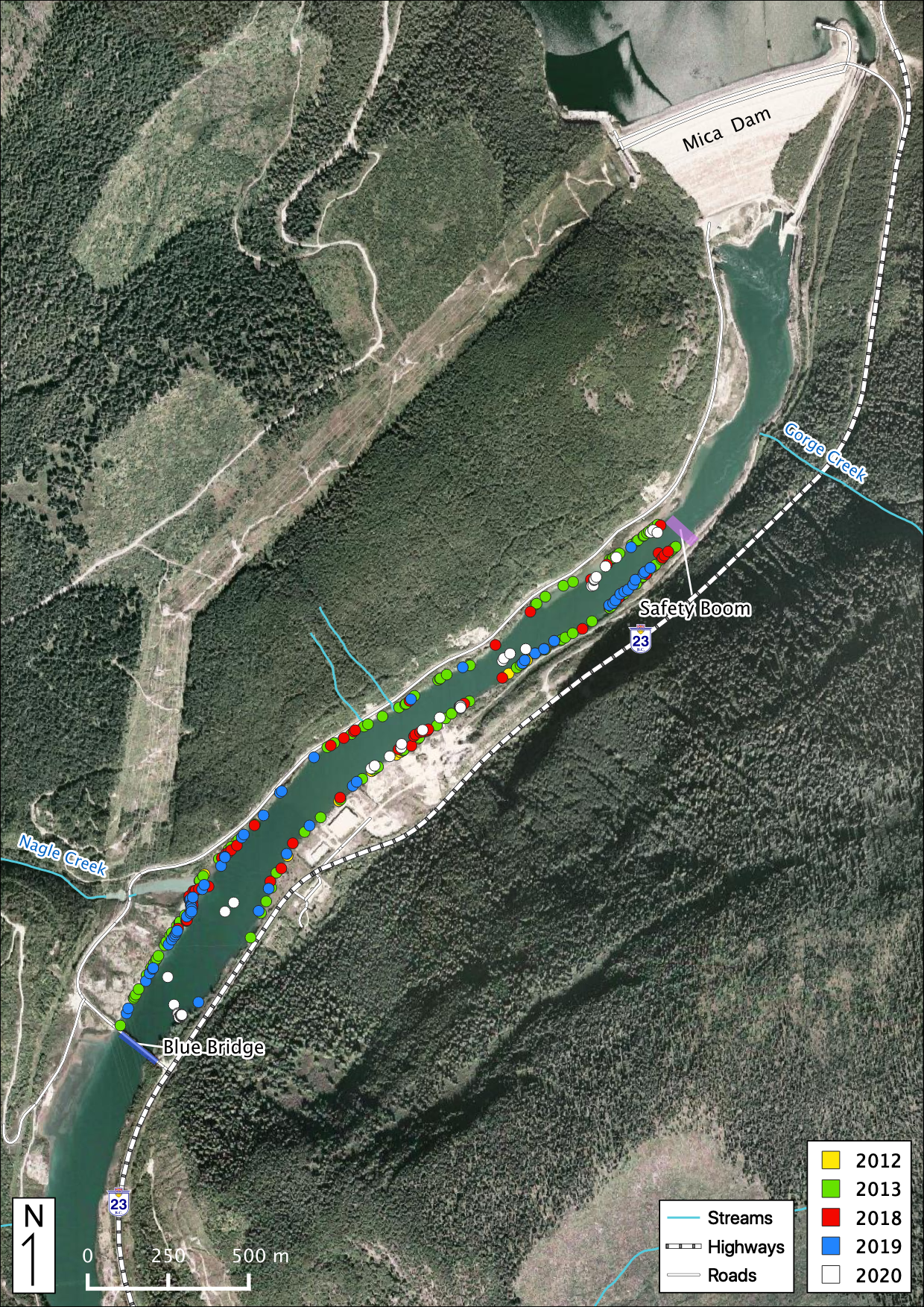
Figure 49. Adult Kokanee observations in the study area below Mica Dam.
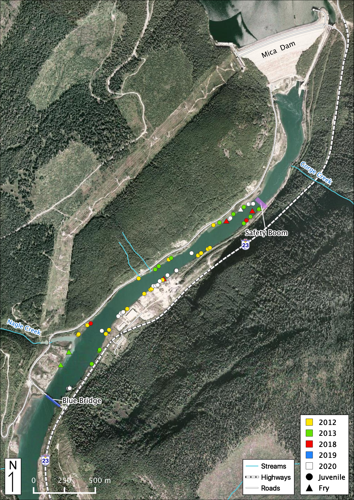
Figure 50. Juvenile and Fry Kokanee observations in the study area below Mica Dam.
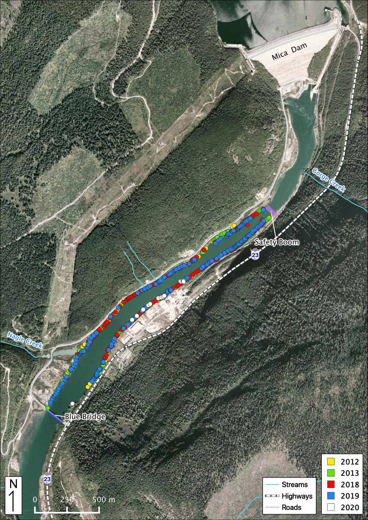
Figure 51. Adult Mountain Whitefish observations in the study area below Mica Dam.
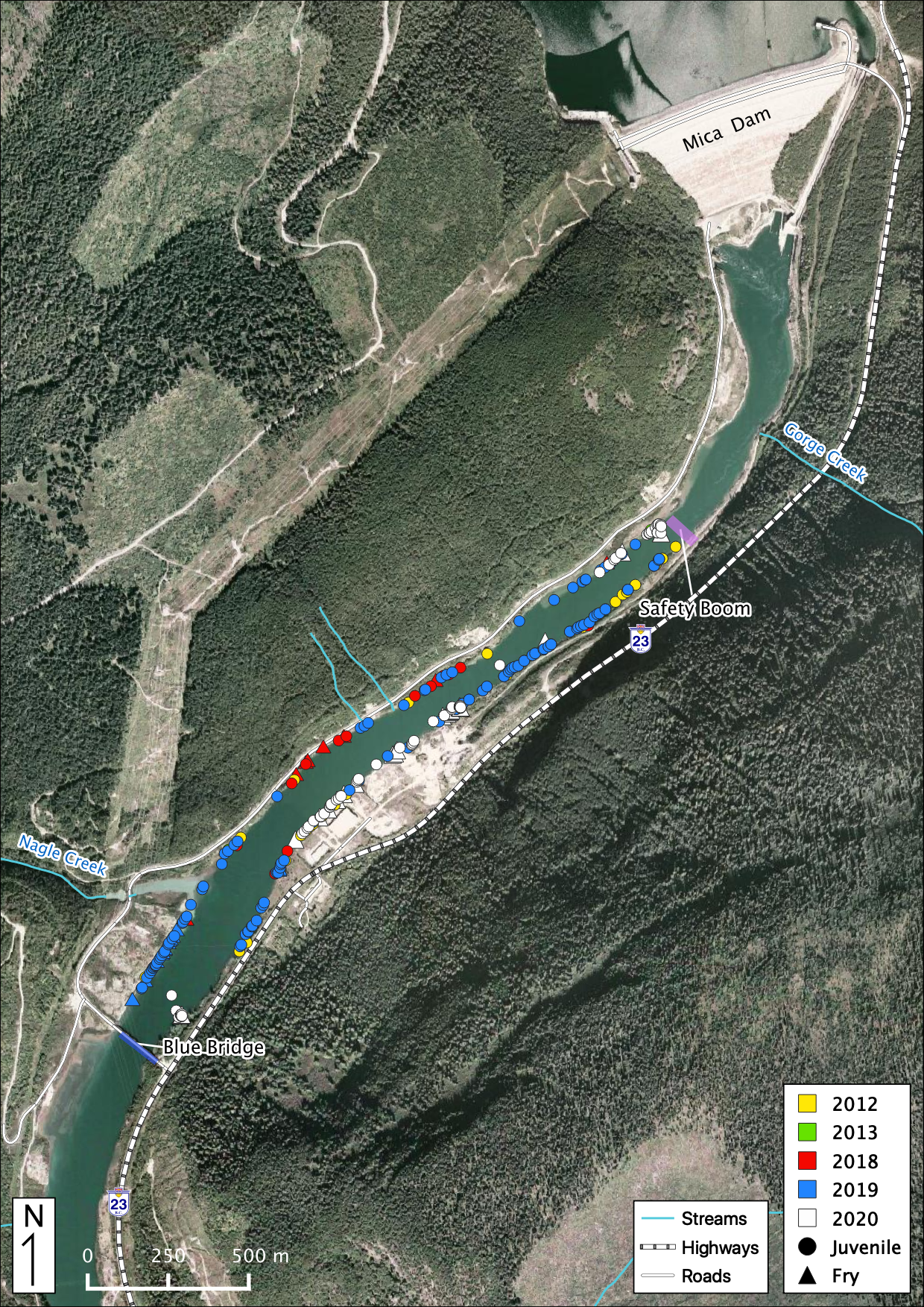
Figure 52. Juvenile and Fry Mountain Whitefish observations in the study area below Mica Dam.
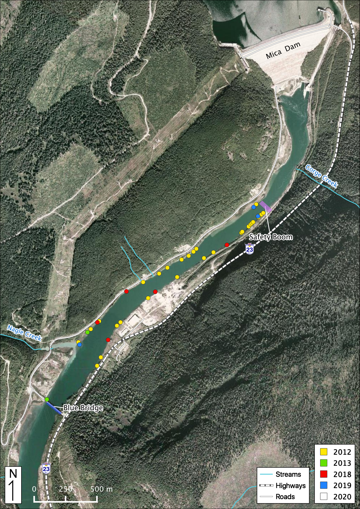
Figure 53. Adult Rainbow Trout observations in the study area below Mica Dam.
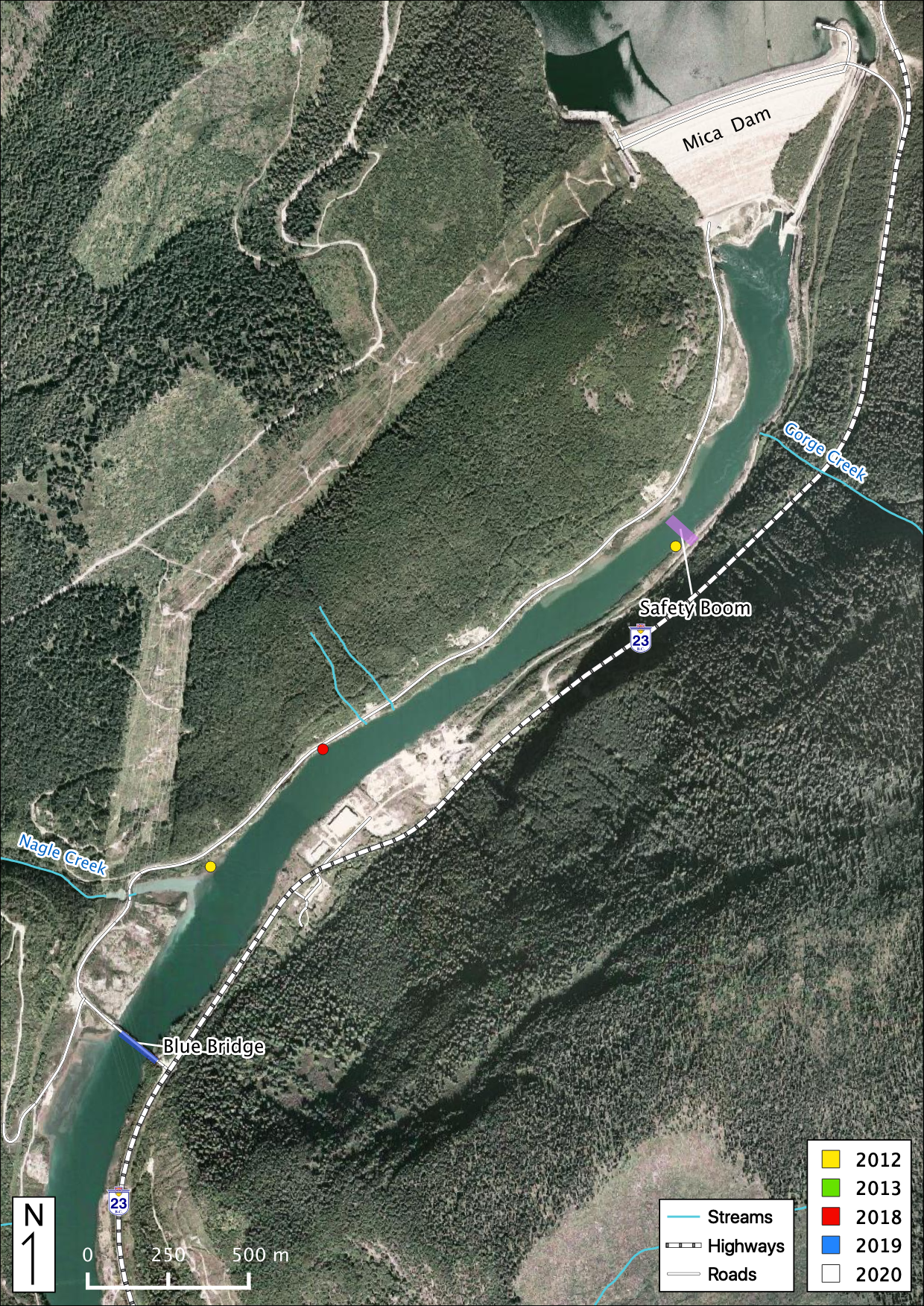
Figure 54. Juvenile Rainbow Trout observations in the study area below Mica Dam.
Acknowledgements
The organisations and individuals whose contributions have made this report possible include:
- BC Hydro
- Trish Joyce
- Jason Watson
- Margo Sadler
- Guy Martel
- Peter McCann
- Fred Katunar
- Alf Leake
- Karen Bray
- Ktunaxa Nation
- Katrina Caley
- Misun Kang
- Joanne Fisher
- Jim Clarricoates
- Bill Green
- Poisson Consulting
- Robyn Irvine
- Seb Dalgarno
- Applied Aquatic Research
- Tom Boag
- Ministry of Forests, Lands and Natural Resource Operations
- Albert Chirico
- Will Warnock
- Jon Bisset
- Mark Thomas
- Charlotte Houston