Mica Dam Expansion Water Temperature and Fish Indexing Study 2019
The suggested citation for this analytic appendix is:
Thorley, J.L. & Amies-Galonski, E. (2020) Mica Dam Expansion Water Temperature and Fish Indexing Study 2019. A Poisson Consulting Analysis Appendix. URL: http://www.poissonconsulting.ca/f/1134568871.
Background
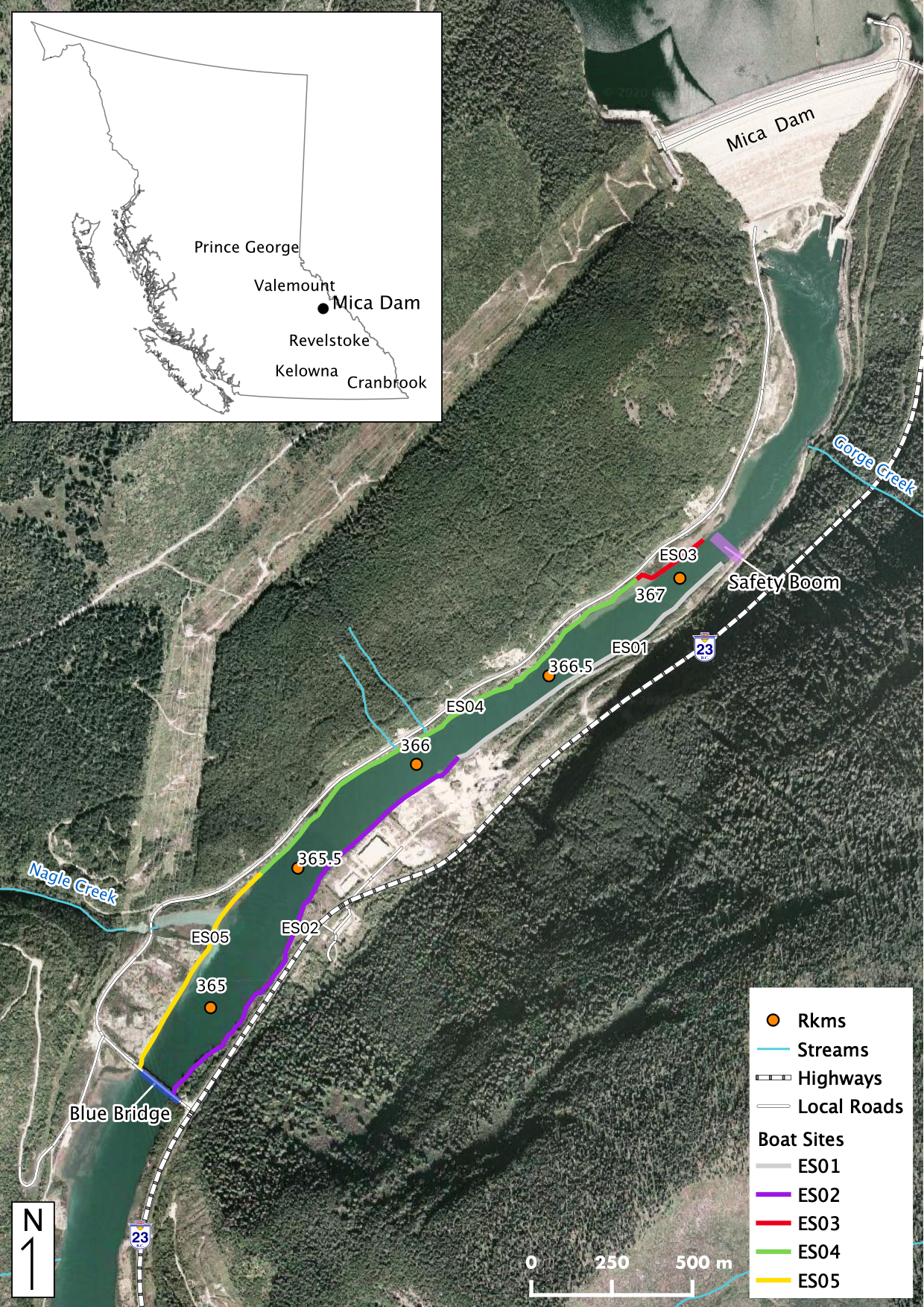
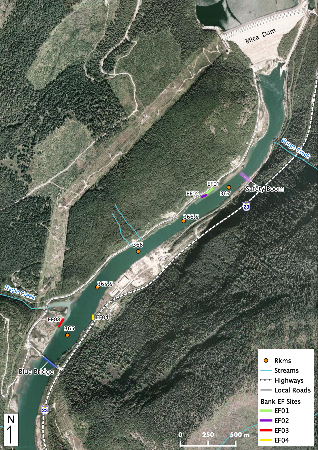
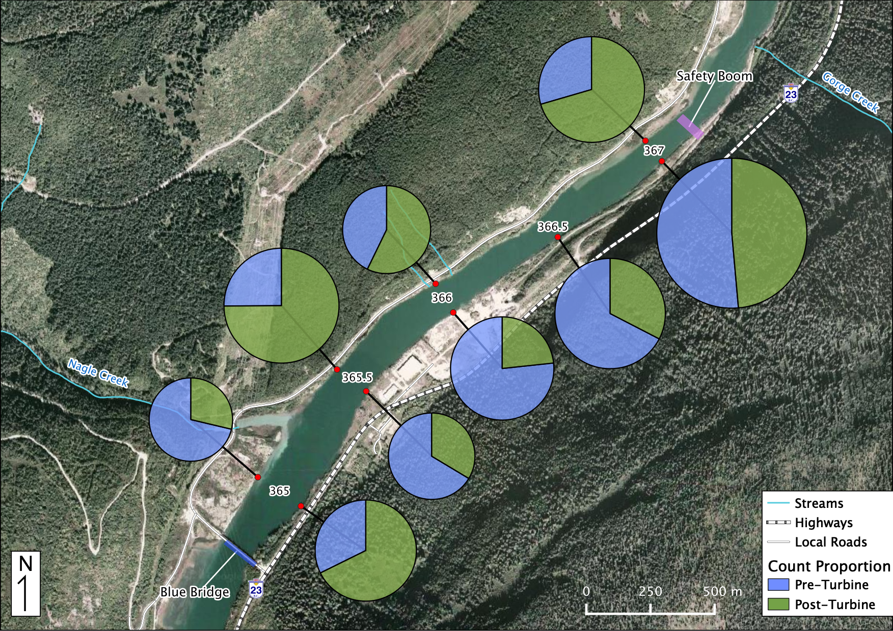
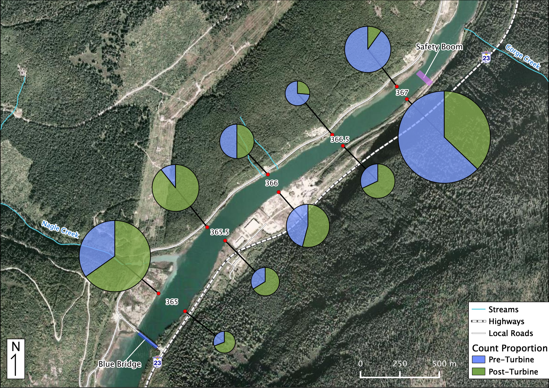
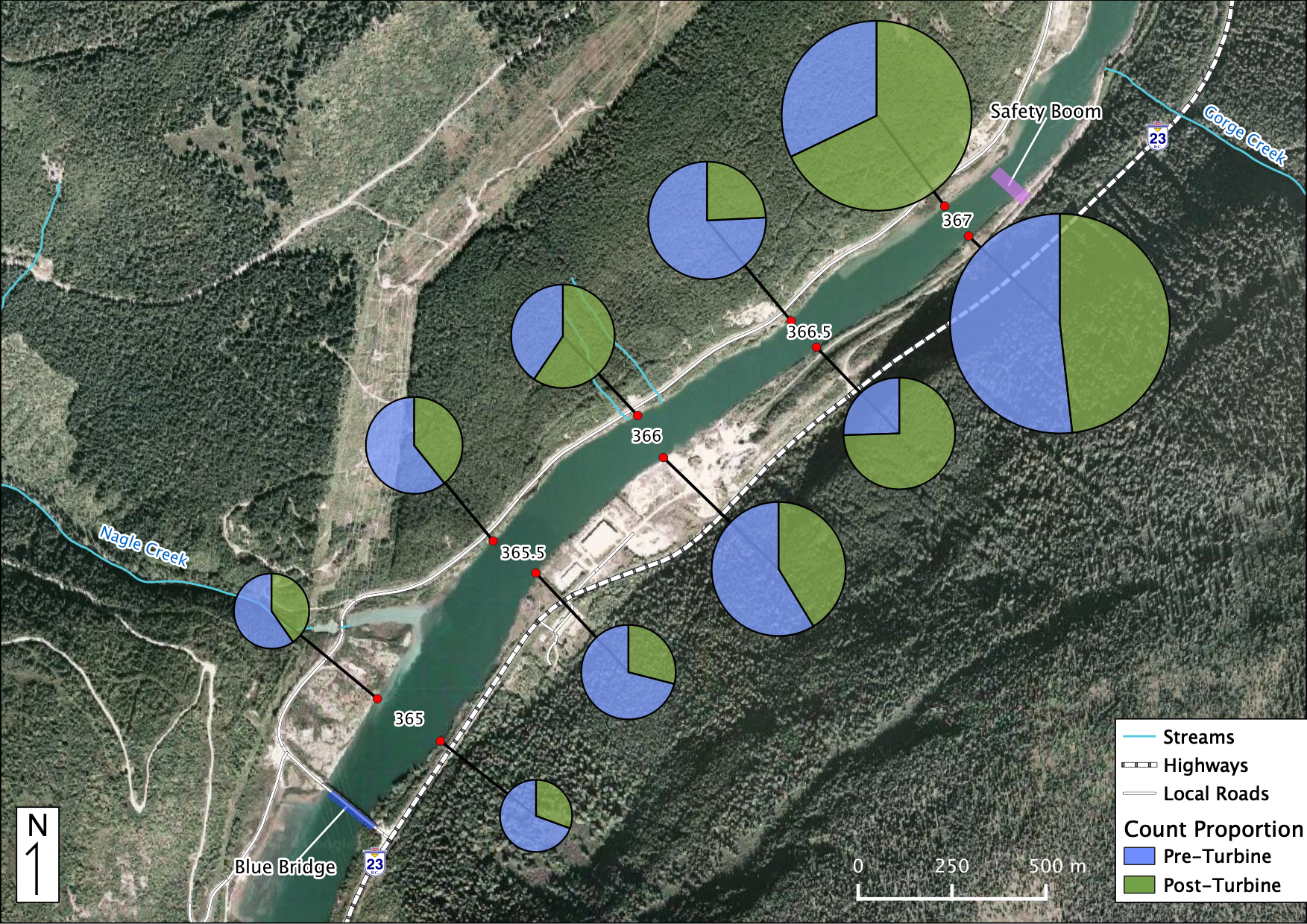
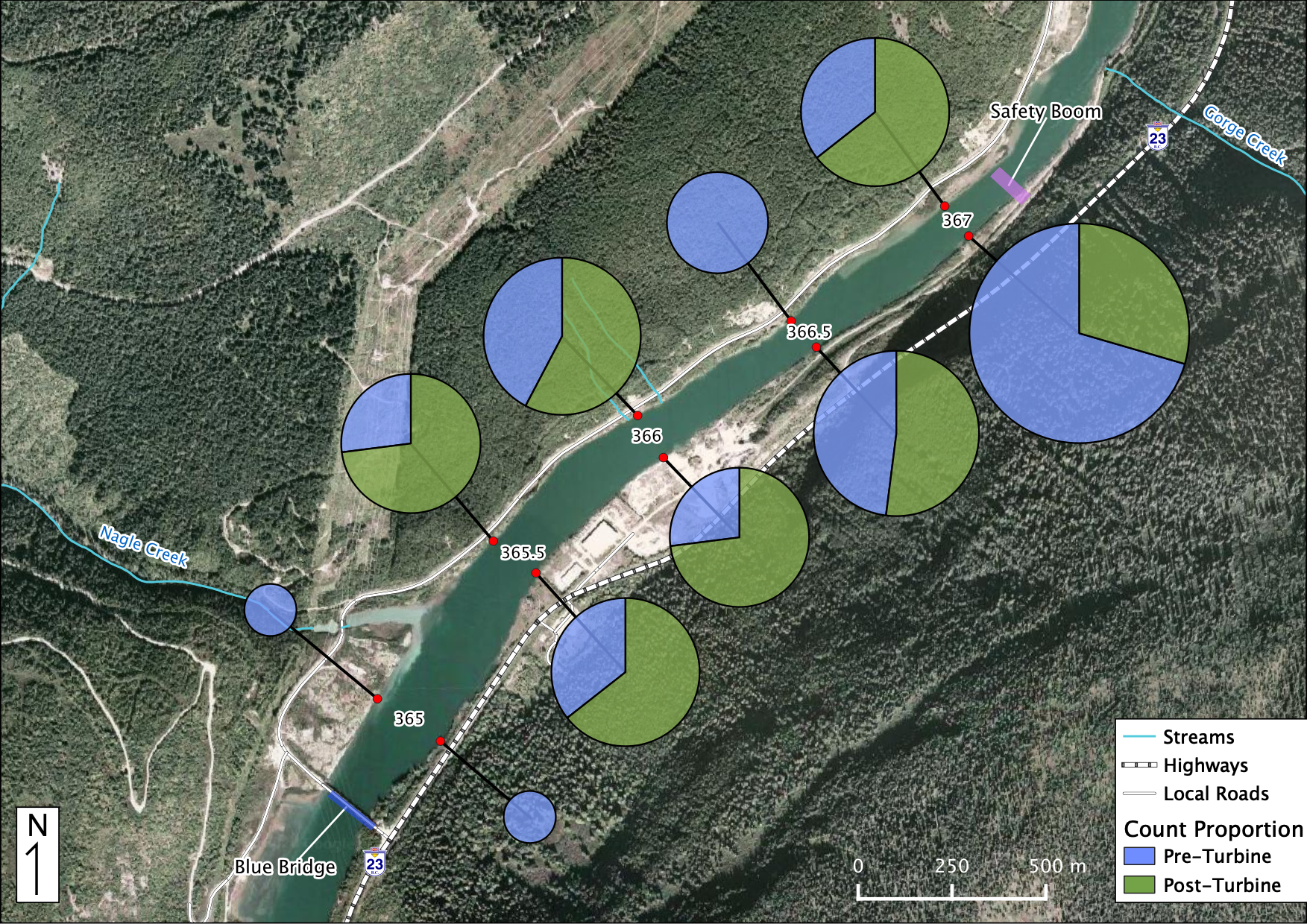
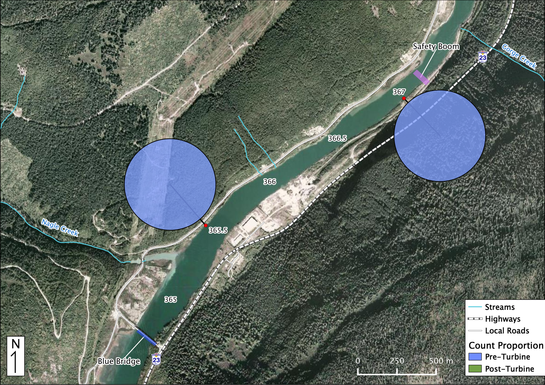
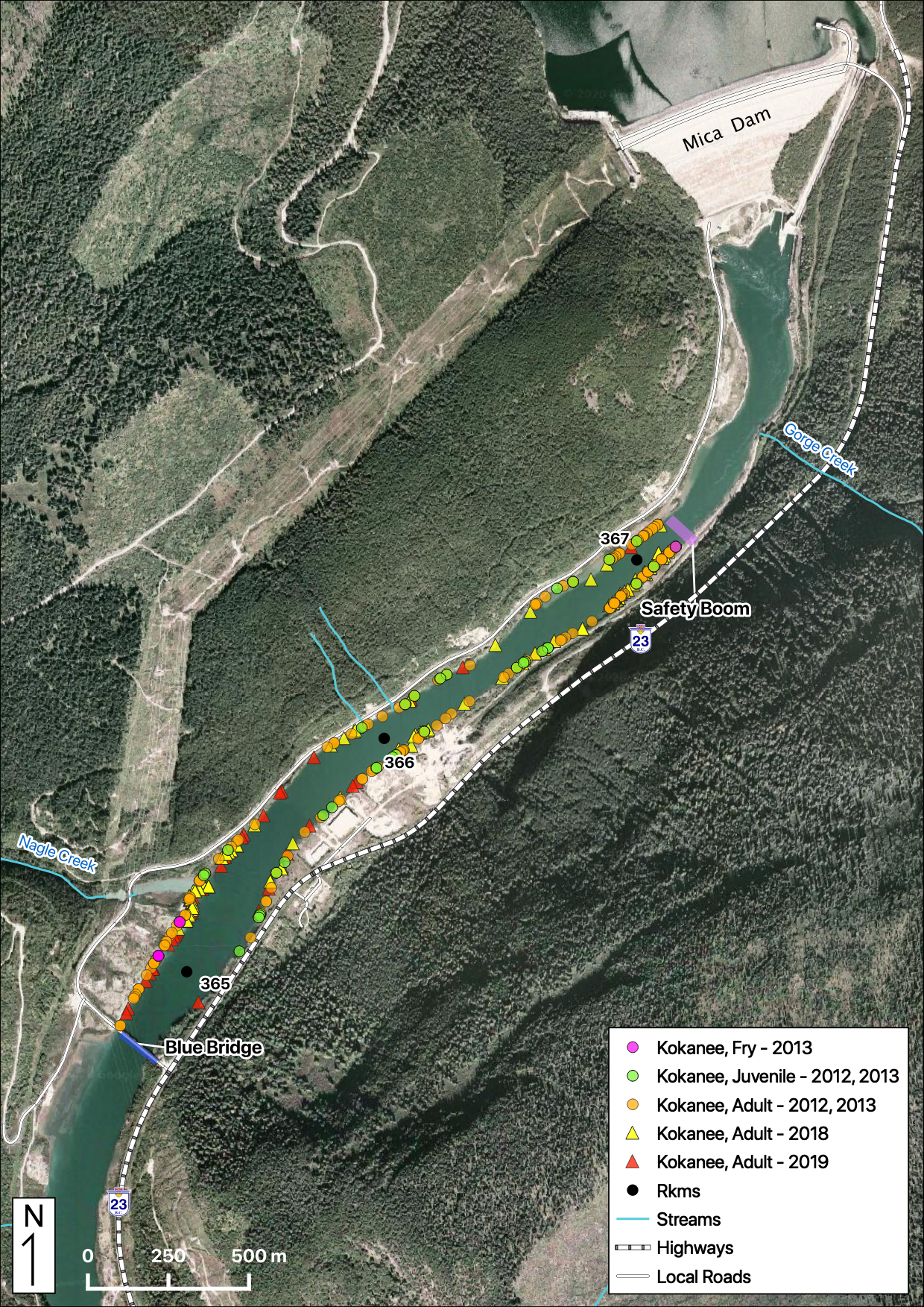
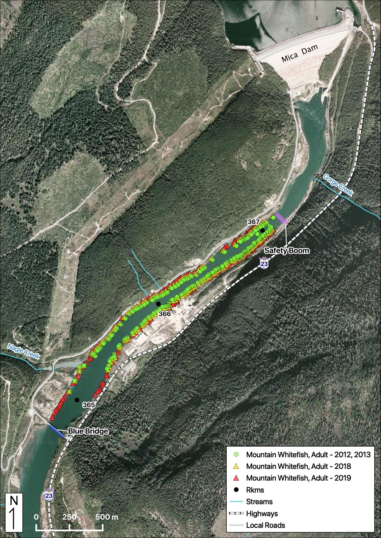
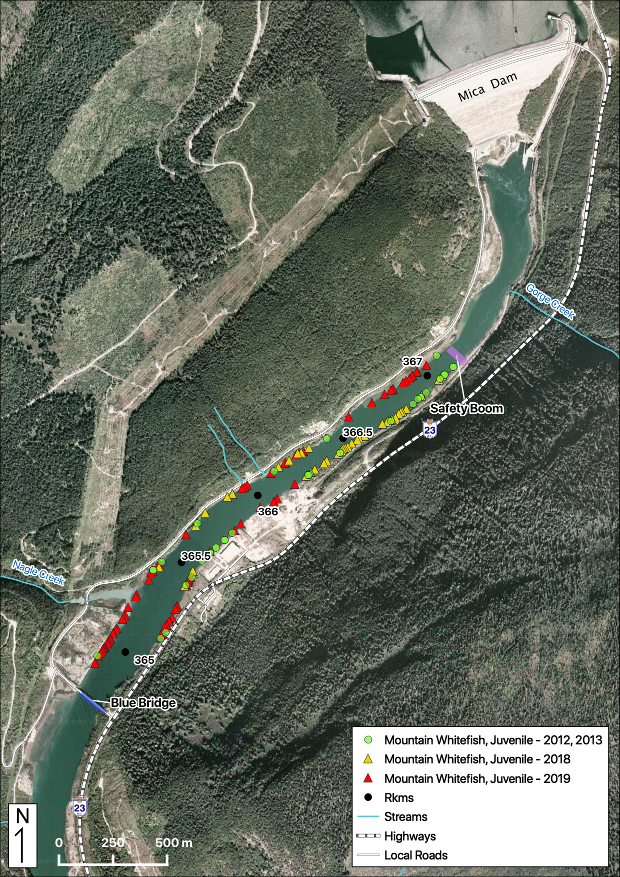
The Mica Tailrace Fish Indexing Study is a multi-year program to estimate the effects of the addition of two new turbines (Mica 5 and 6) on the ichyofauna and thermal regime in the 2.5 km of the Columbia River downstream of Mica Dam. A single year of fish indexing data (2008) was also available from a previous program. As per the Terms of Reference (TOR) the relative abundance, condition and spatial distribution of the fish populations was assessed. In addition, changes in the species evenness were also estimated.
Mica 5 became operational on January 28th 2015 and Mica 6 became operational on December 22nd 2015.
Data Preparation
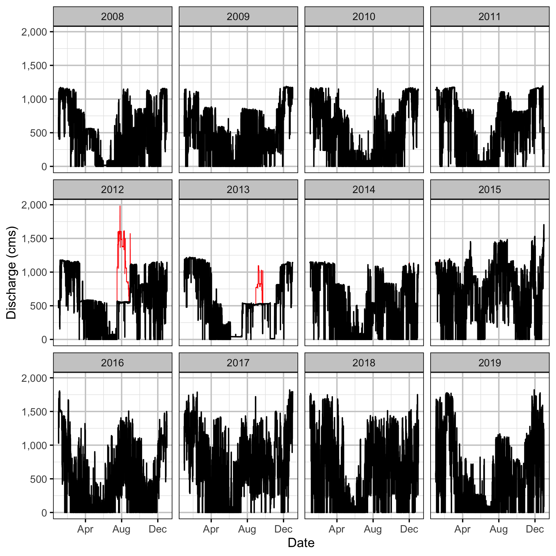
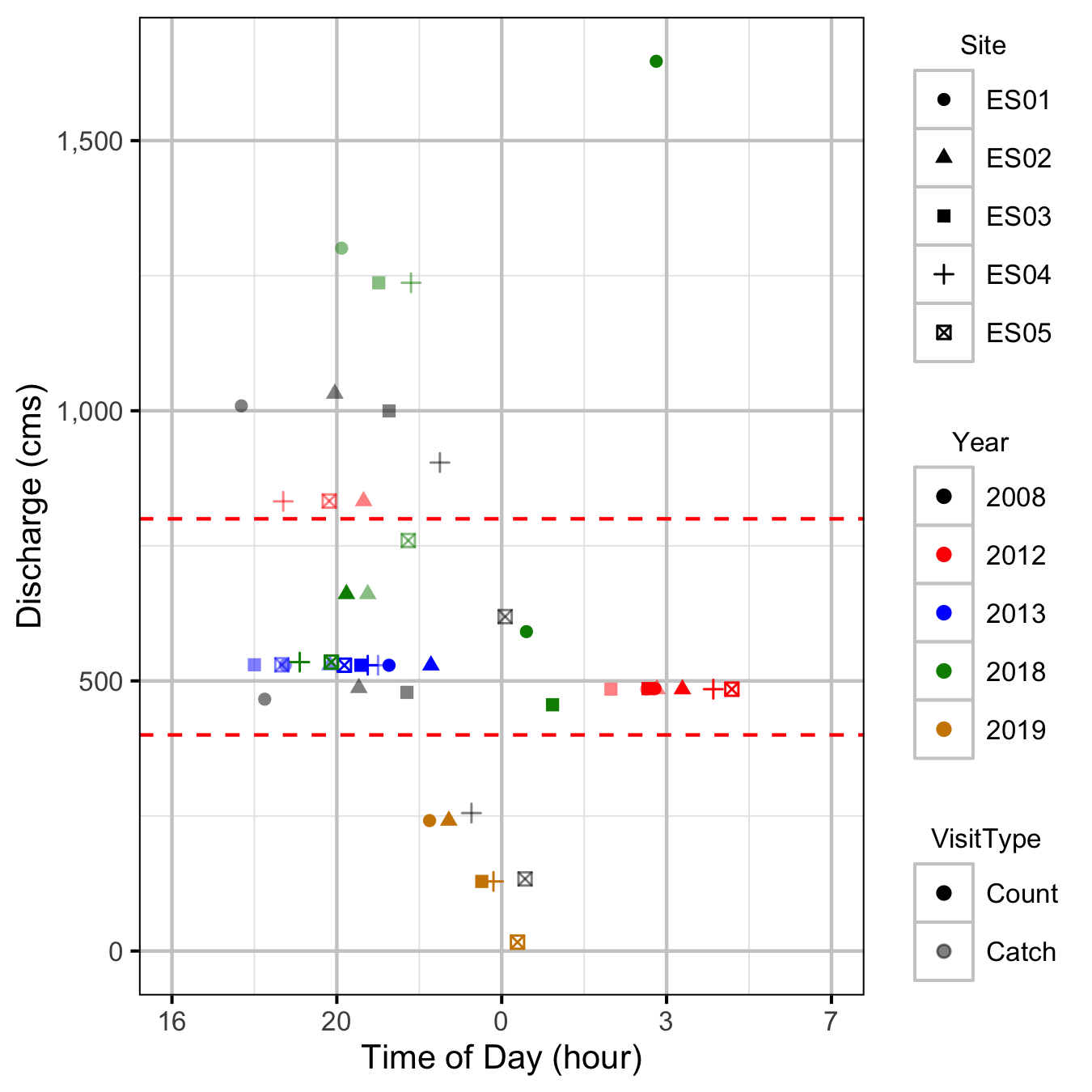
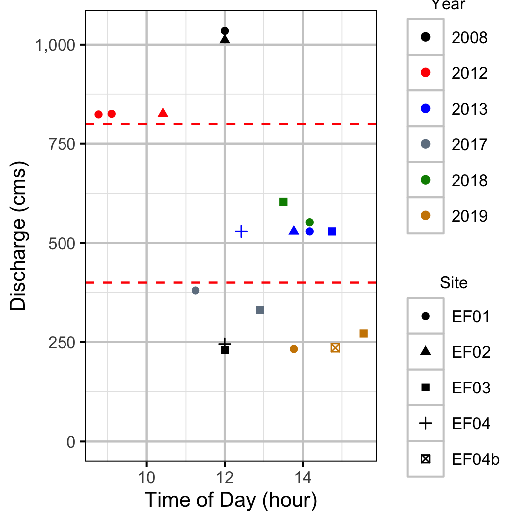
The fish and temperature data were provided by the Ktunaxa Nation. The discharge and elevation data were queried from the Columbia Basin Hydrological Database.
The data were cleaned and tidied using R version 4.0.1 (R Core Team 2015).
Length Cutoffs
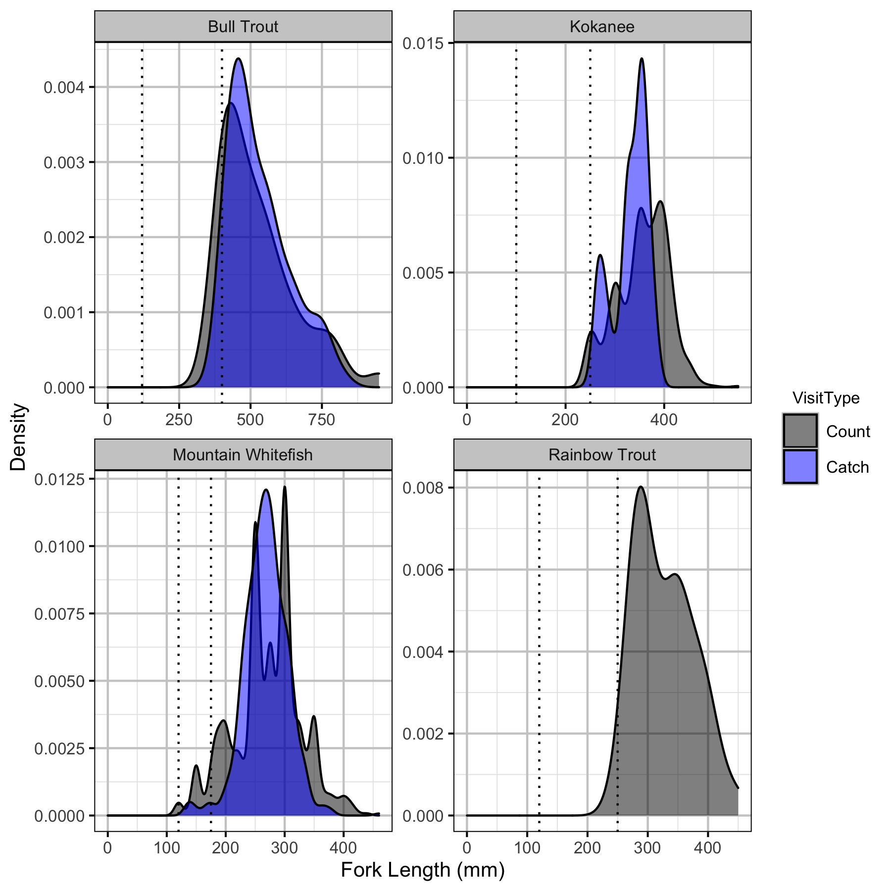
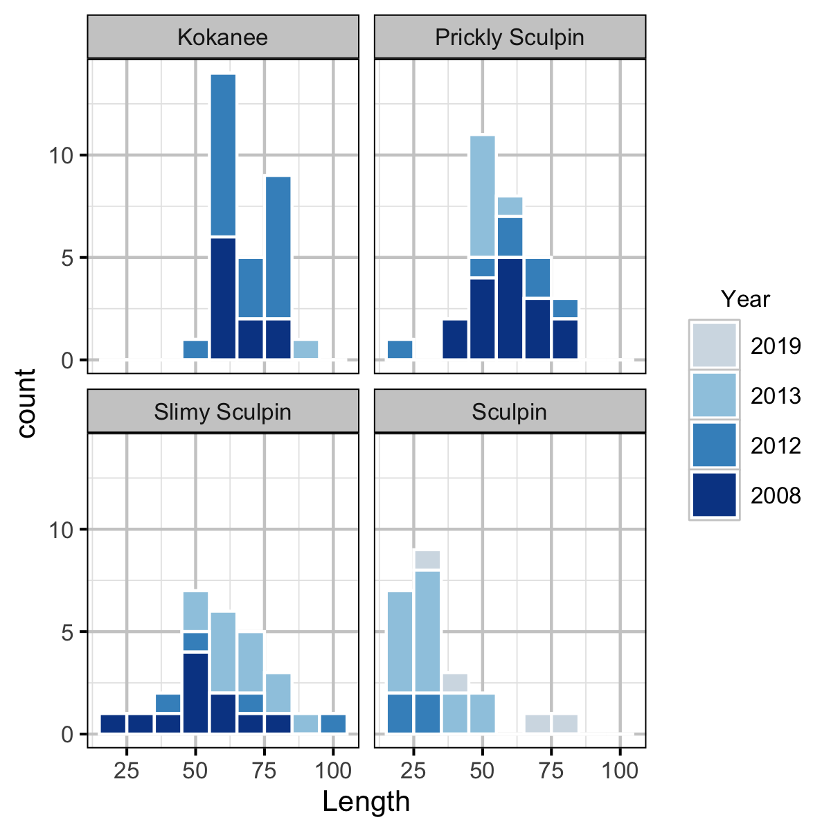
Individuals were classified as fry (age-0), juvenile (age-1 and older subadults) or adult (sexually mature) based on the length cut-offs in Table 1.
Statistical Analysis
Model parameters were estimated using Bayesian methods. The Bayesian estimates were produced using JAGS (Plummer 2015). For additional information on Bayesian estimation the reader is referred to McElreath (2016).
Unless indicated otherwise, the Bayesian analyses used normal and uniform prior distributions that were vague in the sense that they did not constrain the posteriors (Kery and Schaub 2011, 36). The posterior distributions were estimated from 1500 Markov Chain Monte Carlo (MCMC) samples thinned from the second halves of 3 chains (Kery and Schaub 2011, 38–40). Model convergence was confirmed by ensuring that the potential scale reduction factor \(\hat{R} \leq 1.05\) (Kery and Schaub 2011, 40) and the effective sample size (Brooks et al. 2011) \(\textrm{ESS} \geq 150\) for each of the monitored parameters (Kery and Schaub 2011, 61).
The parameters are summarised in terms of the point estimate, standard deviation (sd), the z-score, lower and upper 95% confidence/credible limits (CLs) and the p-value (Kery and Schaub 2011, 37, 42). The estimate is the median (50th percentile) of the MCMC samples, the z-score is \(\mathrm{mean}/\mathrm{sd}\) and the 95% CLs are the 2.5th and 97.5th percentiles. A p-value of 0.05 indicates that the lower or upper 95% CL is 0.
The results are displayed graphically by plotting the modeled relationships between particular variables and the response(s) with the remaining variables held constant. In general, continuous and discrete fixed variables are held constant at their mean and first level values, respectively, while random variables are held constant at their typical values (expected values of the underlying hyperdistributions) (Kery and Schaub 2011, 77–82). When informative the influence of particular variables is expressed in terms of the effect size (i.e., percent change in the response variable) with 95% confidence/credible intervals (CIs, Bradford, Korman, and Higgins 2005).
The analyses were implemented using R version 4.0.1
(R Core Team 2018) and the
mbr family of packages.
Model Descriptions
Body Condition
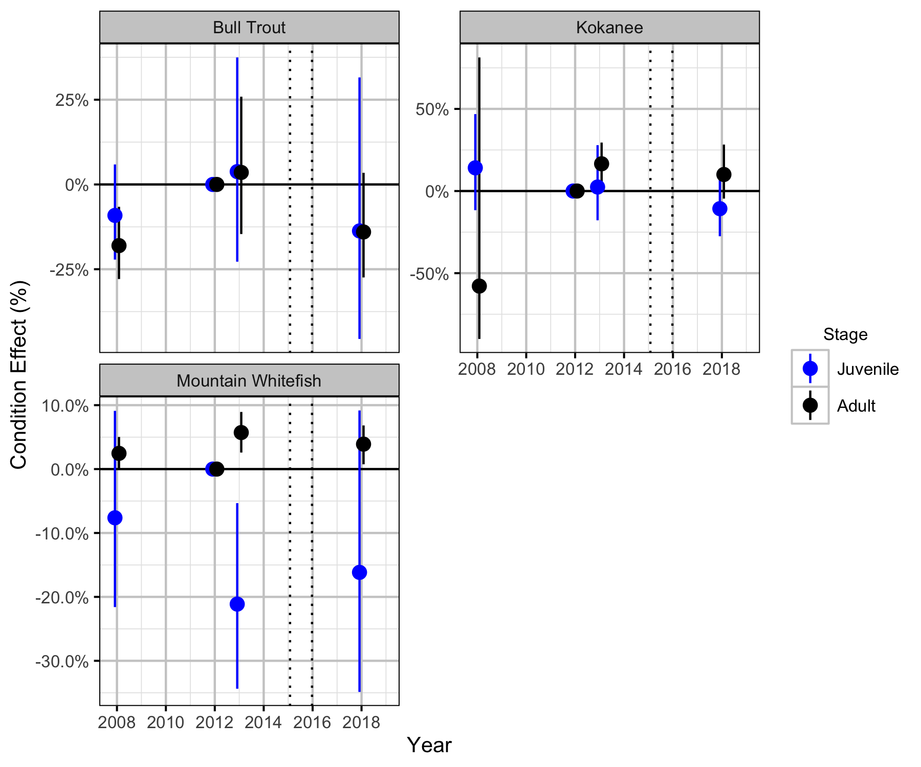
The annual variation in condition (body weight when accounting for body length) was estimated from the boat and backpack electrofishing captures using a mass-length model (He et al. 2008).
Key assumptions of the condition model include:
- Weight varies with body length as an allometric relationship, i.e., \(W = \alpha L^{\beta}\).
- \(\alpha\) varies with year.
- \(\beta\) varies with year.
- The residual variation in weight is log-normally distributed.
Preliminary analyses indicated that site and day of the year were not informative predictors of condition.
Relative Abundance
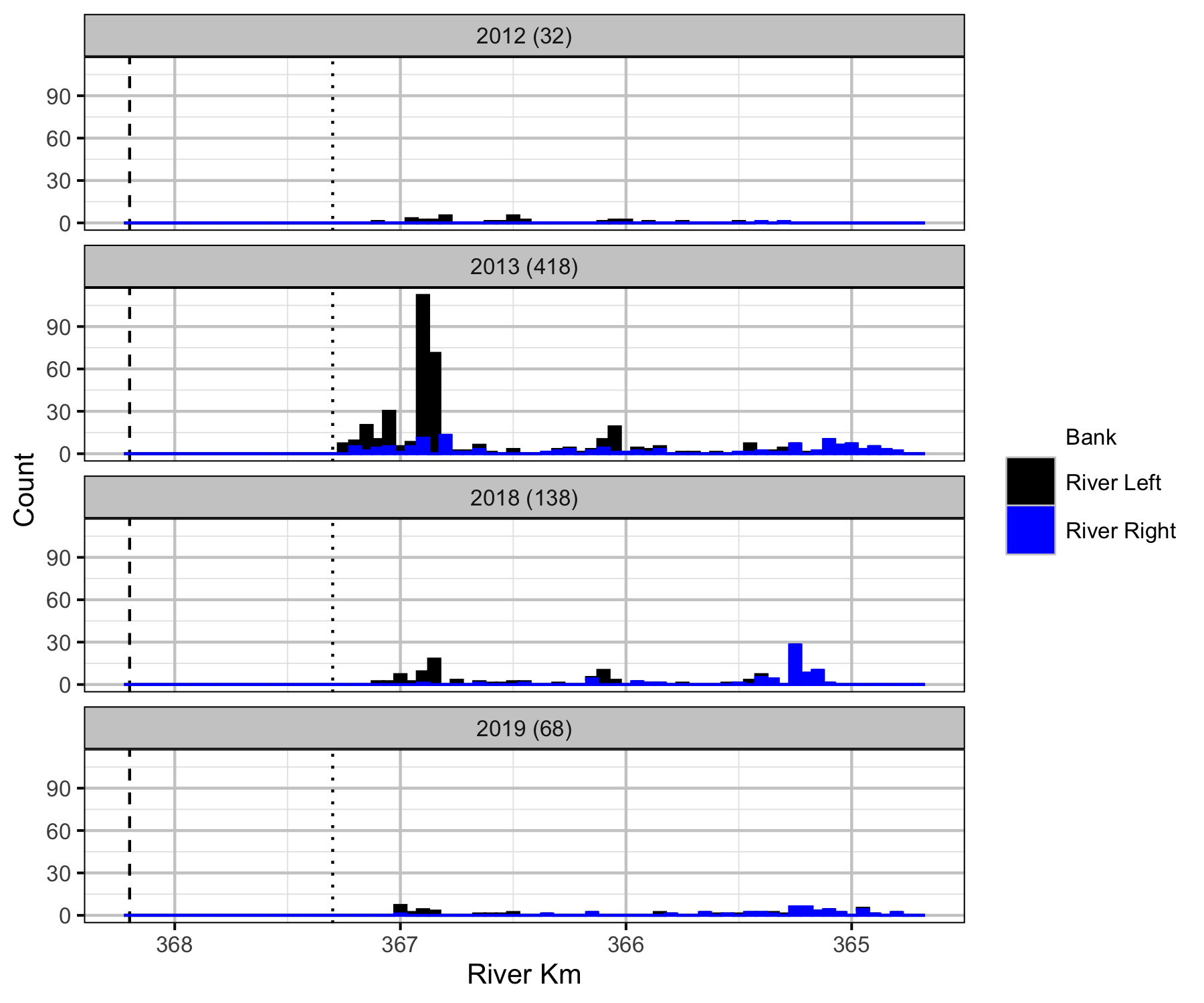
The annual variation in relative abundance was estimated from the boat count and catch data using an over-dispersed Poisson model (Kery and Schaub 2011). Lineal densities are by kilometre of river (as opposed to kilometre of bank).
Key assumptions of the relative abundance model include:
- Lineal density varies by period.
- Lineal density varies randomly with year.
- Lineal catch density is a fixed proportion of lineal count density.
- Expected counts (and catches) are the product of the count (catch) density and the length of river (half the length of bank) sampled.
- Observed counts (and catches) are described by a Poisson-gamma distribution.
Preliminary analyses indicated that site was not an informative predictor of lineal density.
The model does not distinguish between the abundance and observer efficiency, i.e., it estimates the count which is the product of the two. As such it is necessary to assume that changes in observer efficiency by year are negligible in order to interpret the estimates as relative abundance.
Water Temperature
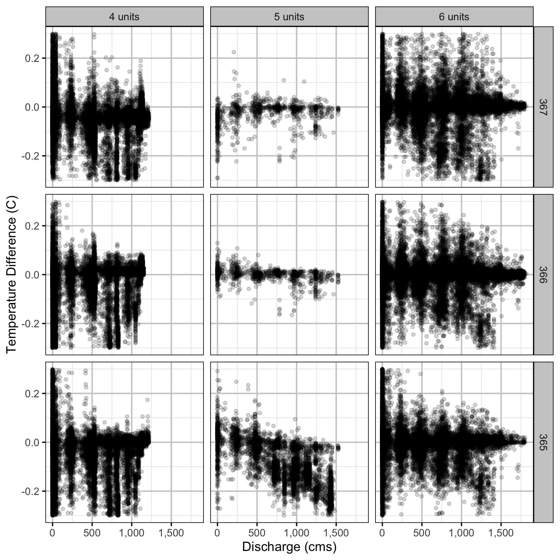
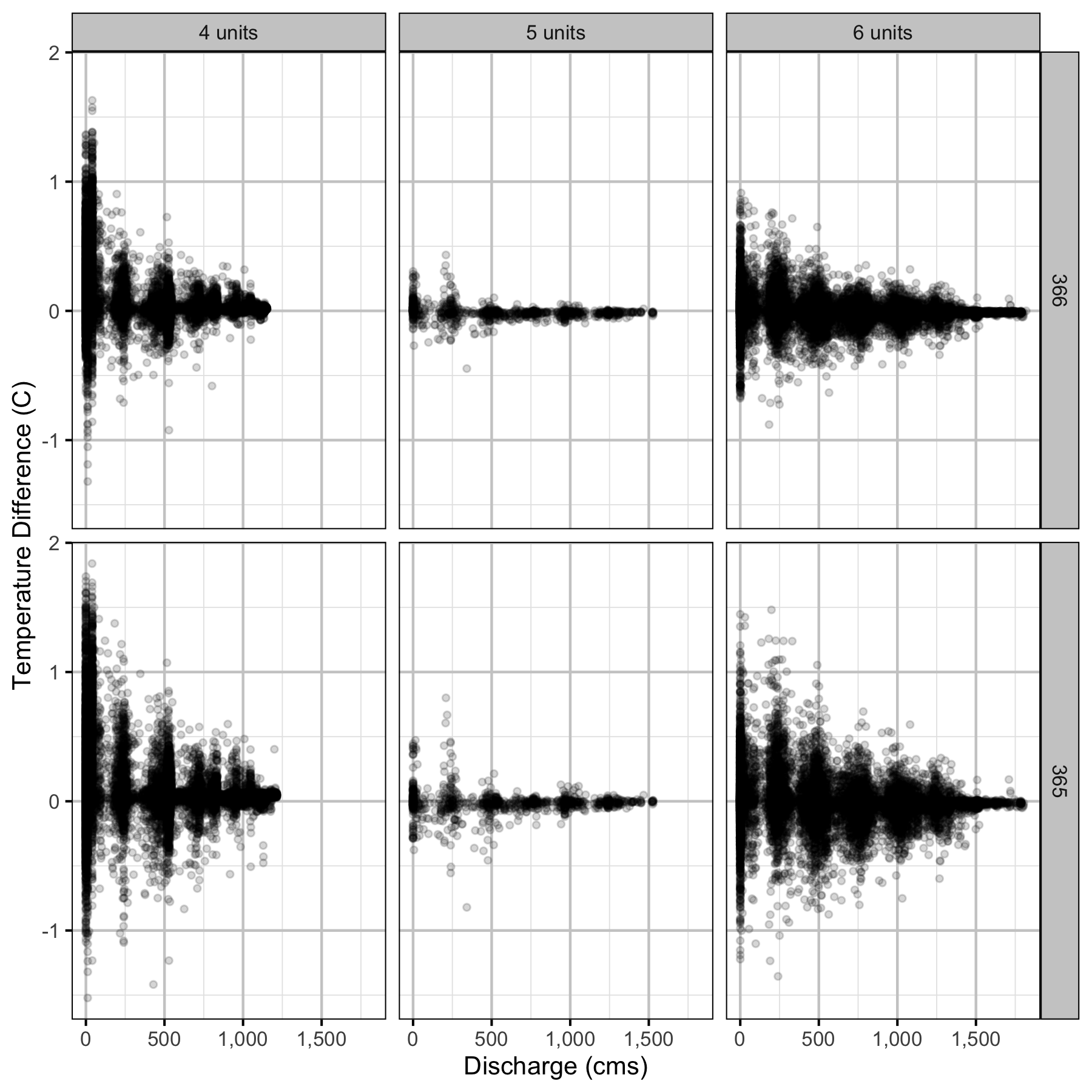
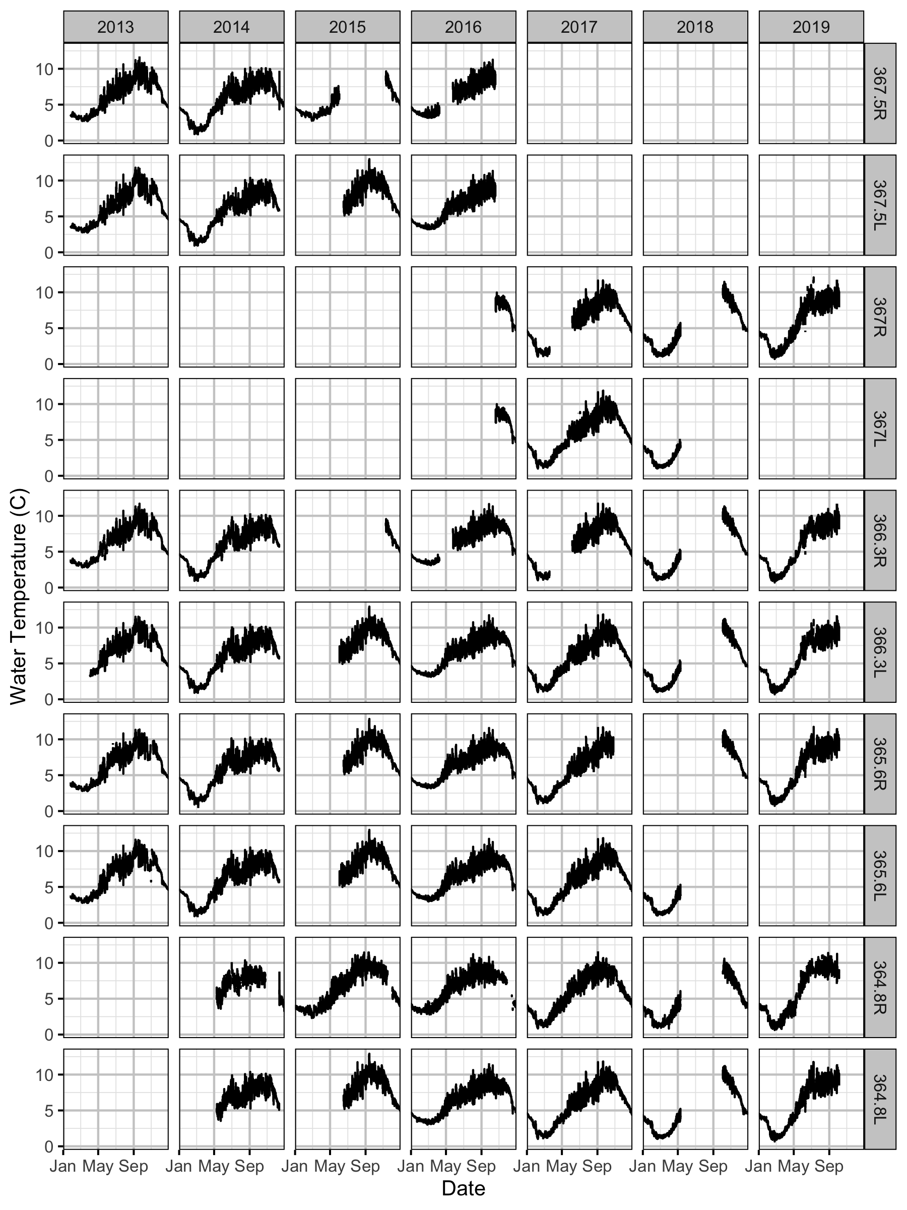
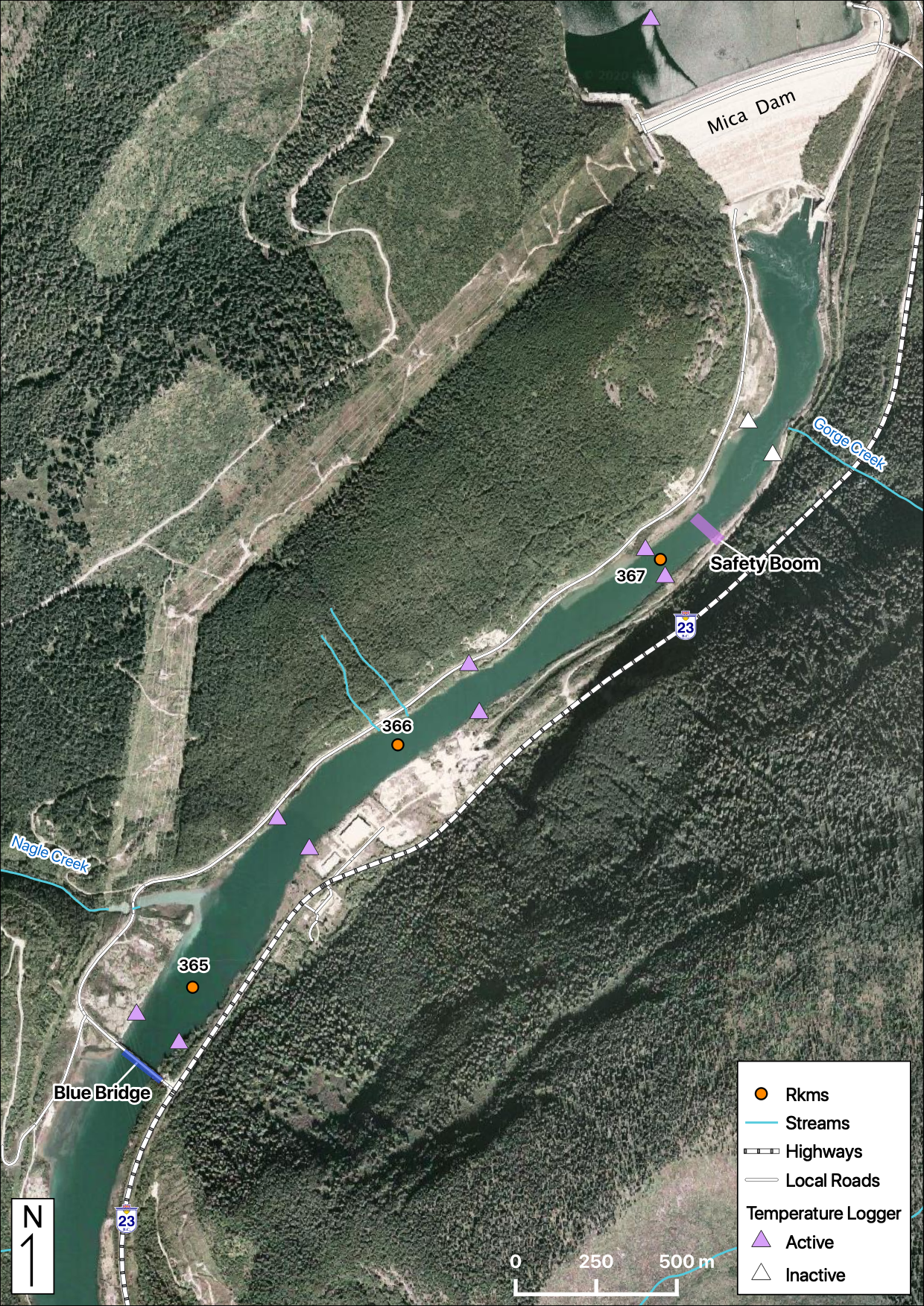
Climatic variation can cause large differences in annual temperatures. Consequently, we explored the data for an effect of the additional turbines on the difference in the water temperature between the right versus left bank and when moving downstream. All apparent systematic differences were within the accuracy of the temperature loggers (\(\pm 0.2^{\circ}\text{C}\)).
Model Templates
Condition
.model{
  bWeightAlpha ~ dnorm(5, 2^-2)
  bWeightBeta ~ dnorm(3, 2^-2)
  bWeightAlphaYear[1] <- 0
  for(i in 2:nYear) {
    bWeightAlphaYear[i] ~ dnorm(0, 2^-2)
  }
  bWeightBetaYear[1] <- 0
  for(i in 2:nYear) {
    bWeightBetaYear[i] ~ dnorm(0, 2^-2)
  }
  sWeight ~ dnorm(0, 2^-2) T(0,)
  for (i in 1:length(Weight)) {
    eWeightAlpha[i] <- bWeightAlpha + bWeightAlphaYear[Year[i]]
    eWeightBeta[i] <- bWeightBeta + bWeightBetaYear[Year[i]]
    log(eWeight[i]) <- eWeightAlpha[i] + eWeightBeta[i] * Length[i]
    Weight[i] ~ dlnorm(log(eWeight[i]), sWeight^-2)
  }
Block 1.
Relative Abundance
.model{
  bEfficiency <- 1
  bEfficiencyVisitType[1] <- 0
  for (i in 2:nVisitType) {
    bEfficiencyVisitType[i] ~ dunif(0, 1)
  }
  bDensity ~ dnorm(0, 5^-2)
  bDensityPeriod[1] <- 0
  for(i in 2:nPeriod) {
    bDensityPeriod[i] ~ dnorm(0, 2^-2)
  }
  sDensityYear ~ dnorm(0, 2^-2) T(0, )
  for(i in 1:nYear) {
    bDensityYear[i] ~ dnorm(0, sDensityYear^-2)
  }
  sDispersion ~ dnorm(0, 2^-2) T(0, )
  for (i in 1:length(Year)) {

    eEfficiency[i] <- bEfficiency - bEfficiencyVisitType[VisitType[i]]
    log(eDensity[i]) <- bDensity + bDensityPeriod[Period[i]] + bDensityYear[Year[i]]
    eAbundance[i] <- eDensity[i] * SiteLength[i] / 2
    eDispersion[i] ~ dgamma(1 / sDispersion^2, 1 / sDispersion^2)
    Count[i] ~ dpois(eAbundance[i] * eEfficiency[i] * eDispersion[i])
  }
Block 2.
Results
Tables
Table 1. Stage Length Cutoffs by Species.
| Species | Fry | Juvenile |
|---|---|---|
| Bull Trout | 120 | 400 |
| Mountain Whitefish | 120 | 175 |
| Rainbow Trout | 120 | 250 |
| Kokanee | 100 | 250 |
Condition
Table 2. Parameter descriptions.
| Parameter | Description |
|---|---|
bWeightAlpha |
Intercept for eAlpha |
bWeightAlphaYear[i] |
Effect of ith Year on eAlpha |
bWeightBeta |
Intercept for eBeta |
bWeightBetaYear[i] |
Effect of ith Year on eBeta |
eAlpha[i] |
Predicted allometric intercept (on centred log
length) for ith fish |
eBeta[i] |
Predicted allometric slope for ith fish |
eWeight[i] |
Predicted weight of ith fish |
Length[i] |
Centred log Length of ith fish |
sWeight |
SD of residual variation in log(Weight) |
Weight[i] |
Weight of ith fish |
Year[i] |
Year of capture of of ith fish |
Bull Trout
Table 3. Model coefficients.
| term | estimate | sd | zscore | lower | upper | pvalue |
|---|---|---|---|---|---|---|
| bWeightAlpha | 6.7449388 | 0.0247983 | 272.0063933 | 6.6966093 | 6.7927562 | 0.0006662 |
| bWeightAlphaYear[2] | 0.1537945 | 0.0472707 | 3.2677351 | 0.0624549 | 0.2518433 | 0.0006662 |
| bWeightAlphaYear[3] | 0.1913102 | 0.0713777 | 2.6761293 | 0.0517245 | 0.3267519 | 0.0139907 |
| bWeightAlphaYear[4] | 0.0031772 | 0.0867638 | 0.0305312 | -0.1664233 | 0.1567937 | 0.9733511 |
| bWeightBeta | 3.0575844 | 0.0762974 | 40.0780567 | 2.9110947 | 3.2025522 | 0.0006662 |
| bWeightBetaYear[2] | 0.1474677 | 0.1585681 | 0.9521226 | -0.1521114 | 0.4512170 | 0.3457695 |
| bWeightBetaYear[3] | 0.1461466 | 0.2390108 | 0.6152690 | -0.3140118 | 0.6426729 | 0.5363091 |
| bWeightBetaYear[4] | 0.1514321 | 0.3616289 | 0.4521290 | -0.5229309 | 0.8884279 | 0.6548967 |
| sWeight | 0.1899506 | 0.0139870 | 13.6456842 | 0.1658411 | 0.2193084 | 0.0006662 |
Table 4. Model summary.
| n | K | nchains | niters | nthin | ess | rhat | converged |
|---|---|---|---|---|---|---|---|
| 106 | 9 | 3 | 500 | 1000 | 1240 | 1.002 | TRUE |
Mountain Whitefish
Table 5. Model coefficients.
| term | estimate | sd | zscore | lower | upper | pvalue |
|---|---|---|---|---|---|---|
| bWeightAlpha | 5.2961725 | 0.0059544 | 889.456113 | 5.2842468 | 5.3082016 | 0.0006662 |
| bWeightAlphaYear[2] | -0.0277357 | 0.0117387 | -2.374274 | -0.0510029 | -0.0046830 | 0.0166556 |
| bWeightAlphaYear[3] | 0.0375127 | 0.0127376 | 2.921893 | 0.0121240 | 0.0619230 | 0.0059960 |
| bWeightAlphaYear[4] | 0.0172917 | 0.0123370 | 1.399918 | -0.0063828 | 0.0406689 | 0.1778814 |
| bWeightBeta | 3.0904454 | 0.0254063 | 121.669058 | 3.0416907 | 3.1419747 | 0.0006662 |
| bWeightBetaYear[2] | -0.0910429 | 0.0696022 | -1.299649 | -0.2219548 | 0.0462926 | 0.1992005 |
| bWeightBetaYear[3] | 0.1669278 | 0.0460264 | 3.624426 | 0.0779921 | 0.2590992 | 0.0006662 |
| bWeightBetaYear[4] | 0.1010421 | 0.0932185 | 1.058267 | -0.0943012 | 0.2740300 | 0.2804797 |
| sWeight | 0.1091740 | 0.0030894 | 35.357695 | 0.1035001 | 0.1156018 | 0.0006662 |
Table 6. Model summary.
| n | K | nchains | niters | nthin | ess | rhat | converged |
|---|---|---|---|---|---|---|---|
| 666 | 9 | 3 | 500 | 1000 | 1436 | 1 | TRUE |
Kokanee
Table 7. Model coefficients.
| term | estimate | sd | zscore | lower | upper | pvalue |
|---|---|---|---|---|---|---|
| bWeightAlpha | 4.1183601 | 0.5538914 | 7.451938 | 3.0454152 | 5.1944731 | 0.0006662 |
| bWeightAlphaYear[2] | 0.5702805 | 0.5552647 | 1.004447 | -0.5200763 | 1.6465351 | 0.3391073 |
| bWeightAlphaYear[3] | 0.6871742 | 0.5540270 | 1.215960 | -0.4114166 | 1.7519429 | 0.2391739 |
| bWeightAlphaYear[4] | 0.5984600 | 0.5561922 | 1.064848 | -0.4794231 | 1.6964302 | 0.2951366 |
| bWeightBeta | 2.6612270 | 0.4324766 | 6.167712 | 1.8108572 | 3.5160638 | 0.0006662 |
| bWeightBetaYear[2] | 0.6675097 | 0.4338728 | 1.524901 | -0.2002297 | 1.5181464 | 0.1379081 |
| bWeightBetaYear[3] | 0.7487141 | 0.4403075 | 1.699720 | -0.1168977 | 1.6070710 | 0.1032645 |
| bWeightBetaYear[4] | 0.8154131 | 0.4425914 | 1.818776 | -0.0646487 | 1.6832351 | 0.0712858 |
| sWeight | 0.2401528 | 0.0117704 | 20.448440 | 0.2188555 | 0.2648829 | 0.0006662 |
Table 8. Model summary.
| n | K | nchains | niters | nthin | ess | rhat | converged |
|---|---|---|---|---|---|---|---|
| 224 | 9 | 3 | 500 | 1000 | 348 | 1.002 | TRUE |
Relative Abundance
Table 9. Parameter descriptions.
| Parameter | Description |
|---|---|
bDensity |
Intercept for log(eDensity) |
bDensityYear[i] |
Effect of ith Year on log(eDensity) |
bEfficiencyVisitType[i] |
Value of log(eEfficiency) for ith VisitType |
Count[i] |
Number of fish counted or captured on ith site visit |
eAbundance[i] |
Predicted relative abundance for ith site visit |
eDensity[i] |
Predicted relative lineal density for ith site visit |
eDispersion[i] |
Predicted over-dispersion for ith site visit |
eEfficiency[i] |
Predicted efficiency relative to counting for ith site visit |
sDispersion |
SD of eDispersion |
SiteLength[i] |
Length of bank surveyed on ith site visit |
VisitType[i] |
Type of ith site visit, i.e., count versus catch |
Year[i] |
Year of ith site visit |
Bull Trout
Table 10. Model coefficients.
| term | estimate | sd | zscore | lower | upper | pvalue |
|---|---|---|---|---|---|---|
| bDensity | -4.5483913 | 0.3275357 | -13.8314625 | -5.1263613 | -3.8404662 | 0.0006662 |
| bDensityPeriod[2] | 0.2374427 | 0.4562055 | 0.4749045 | -0.7523516 | 1.0582628 | 0.5389740 |
| bDensityYear[1] | 0.0434851 | 0.2777674 | 0.3065370 | -0.4161822 | 0.7544030 | 0.7228514 |
| bDensityYear[2] | 0.0024447 | 0.2778457 | 0.0084901 | -0.6117651 | 0.5784625 | 0.9853431 |
| bDensityYear[3] | -0.0781649 | 0.3071506 | -0.5057760 | -0.9298301 | 0.3152702 | 0.5909394 |
| bDensityYear[4] | 0.0088800 | 0.3102782 | 0.1018950 | -0.5685696 | 0.7494457 | 0.9160560 |
| bDensityYear[5] | -0.0034100 | 0.3197221 | -0.0566432 | -0.7464800 | 0.6721996 | 0.9586942 |
| bEfficiencyVisitType[2] | 0.4074703 | 0.1600380 | 2.5065399 | 0.0620530 | 0.6805954 | 0.0006662 |
| sDensityYear | 0.2298812 | 0.3165827 | 0.9837614 | 0.0110697 | 1.0198487 | 0.0006662 |
| sDispersion | 0.6699084 | 0.1253256 | 5.3942209 | 0.4514440 | 0.9393357 | 0.0006662 |
Table 11. Model summary.
| n | K | nchains | niters | nthin | ess | rhat | converged |
|---|---|---|---|---|---|---|---|
| 47 | 10 | 3 | 500 | 300 | 1275 | 1.001 | TRUE |
Mountain Whitefish
Table 12. Model coefficients.
| term | estimate | sd | zscore | lower | upper | pvalue |
|---|---|---|---|---|---|---|
| bDensity | -3.9998553 | 0.6871282 | -5.7399114 | -5.1511511 | -2.4978027 | 0.0019987 |
| bDensityPeriod[2] | 0.4268979 | 0.8479944 | 0.4798337 | -1.2914679 | 2.0425909 | 0.5762825 |
| bDensityYear[1] | -0.0073196 | 0.6416822 | -0.0953173 | -1.5692711 | 1.2080869 | 0.9746835 |
| bDensityYear[2] | -0.0642652 | 0.6142377 | -0.2271524 | -1.6528382 | 0.9890030 | 0.8321119 |
| bDensityYear[3] | -0.0155940 | 0.6210001 | -0.0984553 | -1.4948206 | 1.1158375 | 0.9347102 |
| bDensityYear[4] | -0.2525526 | 0.7023522 | -0.5547476 | -2.0781039 | 0.7669402 | 0.5296469 |
| bDensityYear[5] | 0.3003693 | 0.7209217 | 0.6002241 | -0.8024000 | 2.0763404 | 0.5083278 |
| bEfficiencyVisitType[2] | 0.9336702 | 0.0652125 | 14.0521196 | 0.7608646 | 0.9827258 | 0.0006662 |
| sDensityYear | 0.6012339 | 0.5681324 | 1.2832400 | 0.0274513 | 2.1549447 | 0.0006662 |
| sDispersion | 1.4462137 | 0.2430129 | 6.0276759 | 1.0426073 | 1.9873752 | 0.0006662 |
Table 13. Model summary.
| n | K | nchains | niters | nthin | ess | rhat | converged |
|---|---|---|---|---|---|---|---|
| 47 | 10 | 3 | 500 | 300 | 871 | 1.003 | TRUE |
Table 14. Model coefficients.
| term | estimate | sd | zscore | lower | upper | pvalue |
|---|---|---|---|---|---|---|
| bDensity | -1.2081265 | 0.4729651 | -2.4990591 | -1.9980132 | -0.2001549 | 0.0233178 |
| bDensityPeriod[2] | -0.0010120 | 0.6868463 | -0.0526711 | -1.5154086 | 1.2675274 | 0.9986676 |
| bDensityYear[1] | 0.1710568 | 0.4484460 | 0.5043951 | -0.6510449 | 1.2310244 | 0.5629580 |
| bDensityYear[2] | -0.0890931 | 0.4265791 | -0.2839872 | -1.0715728 | 0.6931258 | 0.7521652 |
| bDensityYear[3] | -0.1307897 | 0.4559763 | -0.3856545 | -1.1574369 | 0.7151188 | 0.7268488 |
| bDensityYear[4] | 0.3903445 | 0.5622053 | 0.8114263 | -0.5389353 | 1.8028275 | 0.3644237 |
| bDensityYear[5] | -0.3652971 | 0.5798686 | -0.7599976 | -1.7969391 | 0.5782719 | 0.3764157 |
| bEfficiencyVisitType[2] | 0.7920571 | 0.0757220 | 10.2928288 | 0.5893424 | 0.8896675 | 0.0006662 |
| sDensityYear | 0.5837329 | 0.4369668 | 1.5495358 | 0.0764352 | 1.8190535 | 0.0006662 |
| sDispersion | 0.8079563 | 0.0889596 | 9.1376155 | 0.6580172 | 1.0056799 | 0.0006662 |
Table 15. Model summary.
| n | K | nchains | niters | nthin | ess | rhat | converged |
|---|---|---|---|---|---|---|---|
| 47 | 10 | 3 | 500 | 300 | 226 | 1.016 | TRUE |
Rainbow Trout
Table 16. Model coefficients.
| term | estimate | sd | zscore | lower | upper | pvalue |
|---|---|---|---|---|---|---|
| bDensity | -5.2409836 | 0.9294088 | -5.6698277 | -7.1337351 | -3.5049568 | 0.0006662 |
| bDensityPeriod[2] | -0.8827318 | 1.1774497 | -0.7279018 | -3.0024553 | 1.6377676 | 0.4270486 |
| bDensityYear[1] | 0.2251140 | 1.1755007 | 0.2203285 | -2.1209930 | 2.6264584 | 0.8121252 |
| bDensityYear[2] | 0.9714359 | 0.9350035 | 1.0558831 | -0.7758965 | 2.9116305 | 0.2644903 |
| bDensityYear[3] | -1.1767884 | 1.0787730 | -1.2194615 | -3.6498930 | 0.4372475 | 0.1632245 |
| bDensityYear[4] | -0.0719036 | 1.0643474 | -0.1310672 | -2.5849614 | 1.8924375 | 0.9320453 |
| bDensityYear[5] | -0.2923180 | 1.1039778 | -0.3583067 | -2.8157443 | 1.6691879 | 0.6948701 |
| bEfficiencyVisitType[2] | 0.9819937 | 0.0287034 | 33.9186002 | 0.8962625 | 0.9982746 | 0.0006662 |
| sDensityYear | 1.3086579 | 0.7446227 | 1.9292106 | 0.3619239 | 3.3089916 | 0.0006662 |
| sDispersion | 0.6939334 | 0.3209207 | 2.3315279 | 0.2616054 | 1.4923112 | 0.0006662 |
Table 17. Model summary.
| n | K | nchains | niters | nthin | ess | rhat | converged |
|---|---|---|---|---|---|---|---|
| 47 | 10 | 3 | 500 | 300 | 1326 | 1.003 | TRUE |
Kokanee
Table 18. Model coefficients.
| term | estimate | sd | zscore | lower | upper | pvalue |
|---|---|---|---|---|---|---|
| bDensity | -2.6582197 | 1.0064719 | -2.5979870 | -4.4954955 | -0.3376729 | 0.0366422 |
| bDensityPeriod[2] | -0.5358329 | 1.1167043 | -0.4663438 | -2.8458772 | 1.6139544 | 0.5936043 |
| bDensityYear[1] | -0.9169311 | 1.0064755 | -1.0125952 | -3.2711543 | 0.7346803 | 0.2245170 |
| bDensityYear[2] | 0.8553464 | 0.9959584 | 0.8460199 | -1.2940564 | 2.7062580 | 0.3057961 |
| bDensityYear[3] | 0.0329223 | 0.9904930 | -0.0244477 | -2.2107747 | 1.8996879 | 0.9720187 |
| bDensityYear[4] | -0.1216088 | 1.0062846 | -0.1714605 | -2.4059291 | 1.7498253 | 0.8800799 |
| bEfficiencyVisitType[2] | 0.6767797 | 0.1447751 | 4.4805587 | 0.2570010 | 0.8543102 | 0.0006662 |
| sDensityYear | 1.1835941 | 0.7487135 | 1.8104093 | 0.4240694 | 3.2462607 | 0.0006662 |
| sDispersion | 0.9973497 | 0.1321665 | 7.6025711 | 0.7737543 | 1.2995119 | 0.0006662 |
Table 19. Model summary.
| n | K | nchains | niters | nthin | ess | rhat | converged |
|---|---|---|---|---|---|---|---|
| 37 | 9 | 3 | 500 | 300 | 190 | 1.043 | TRUE |
Figures
Discharge
Condition
Relative Abundance
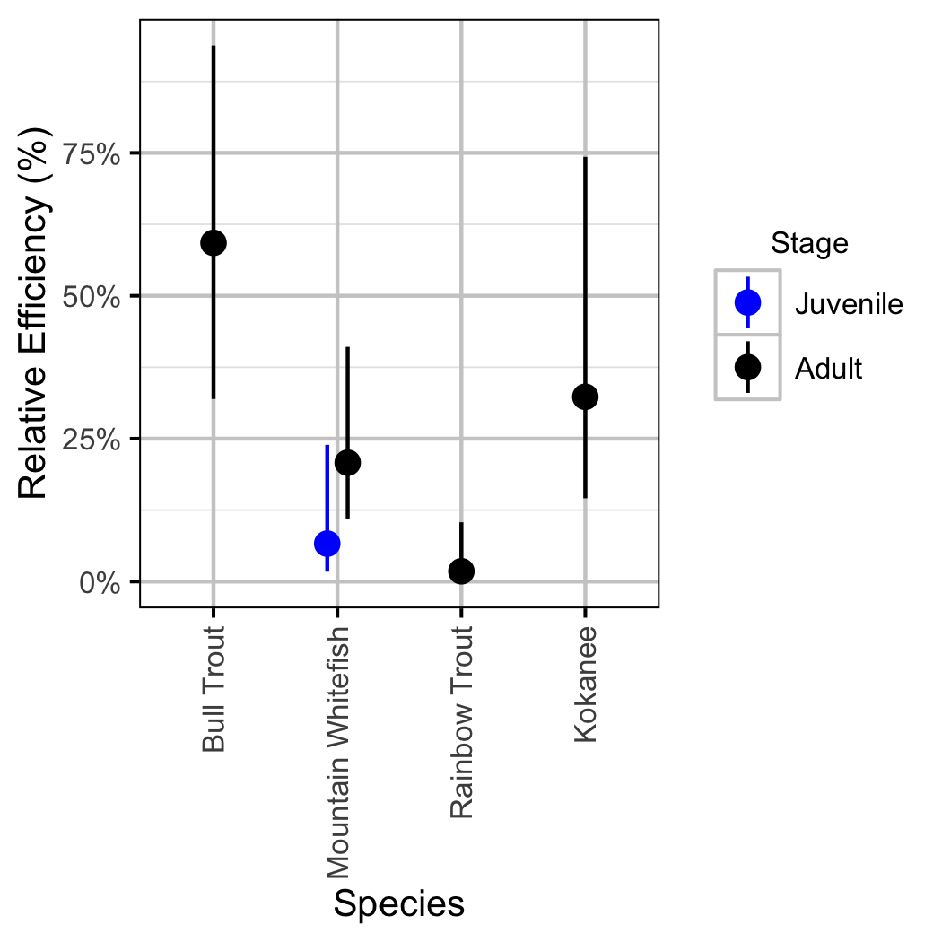
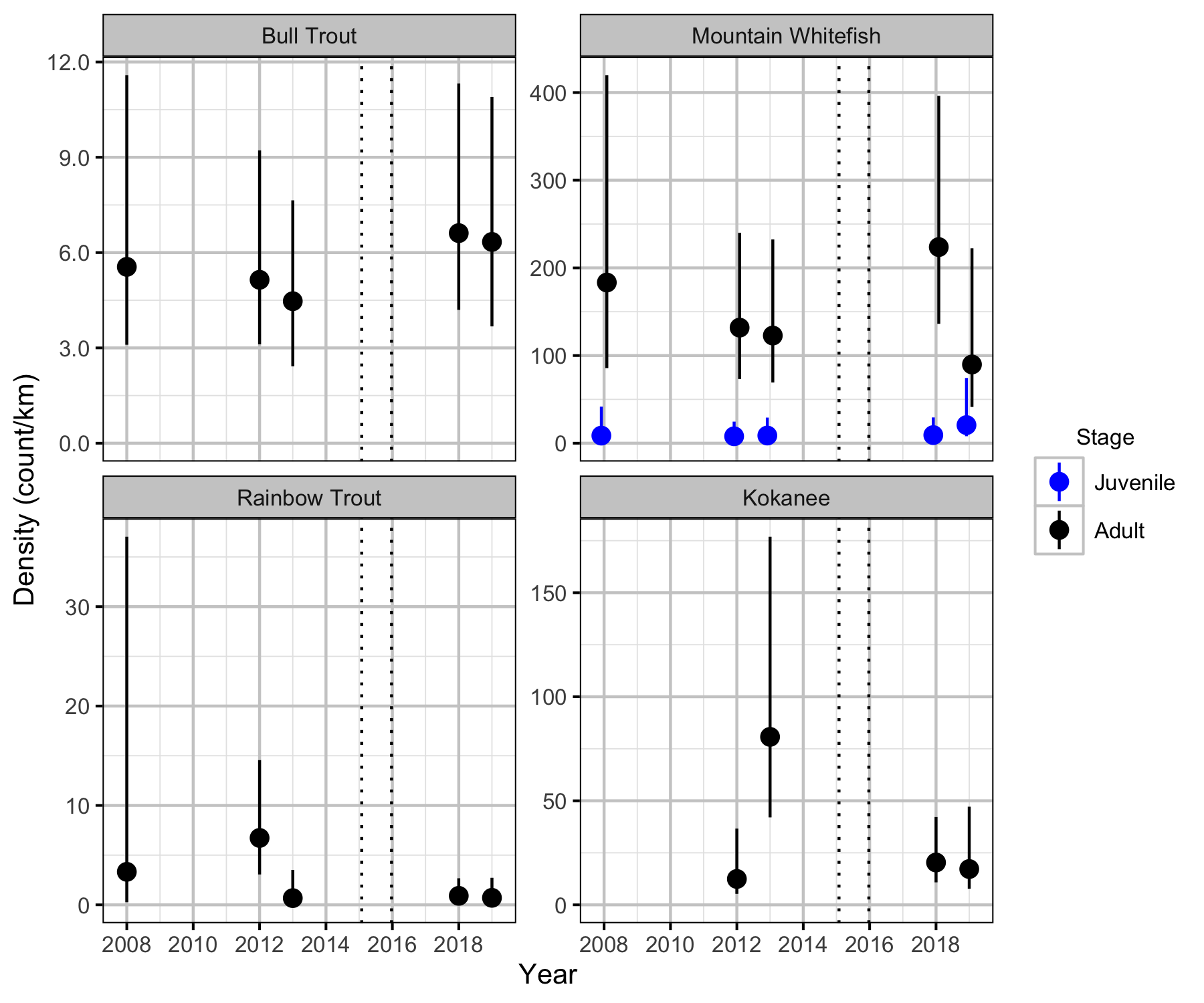
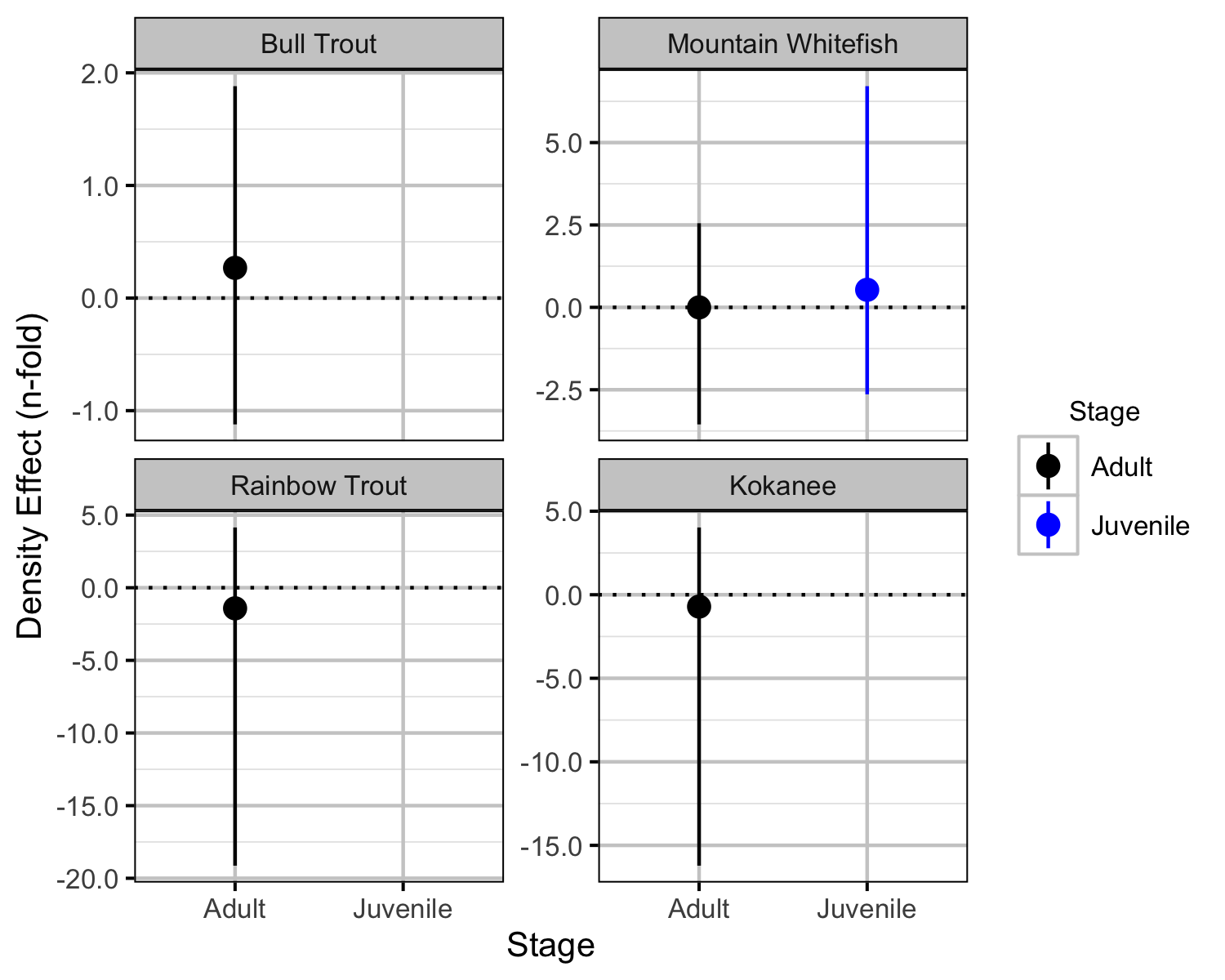
Boat
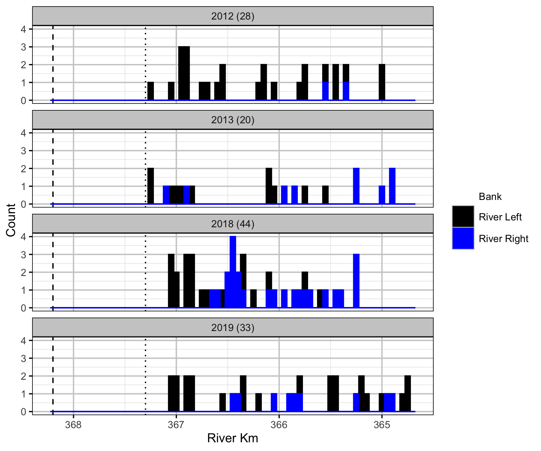
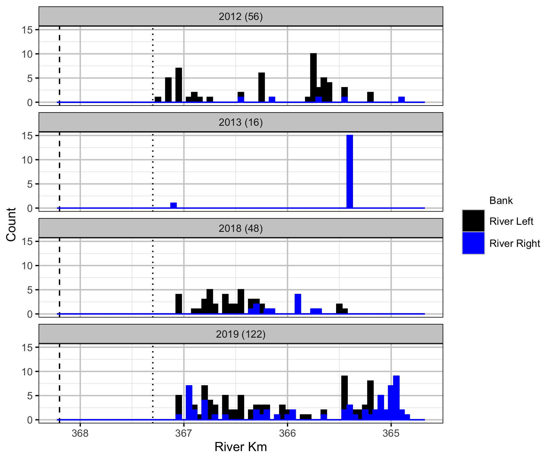
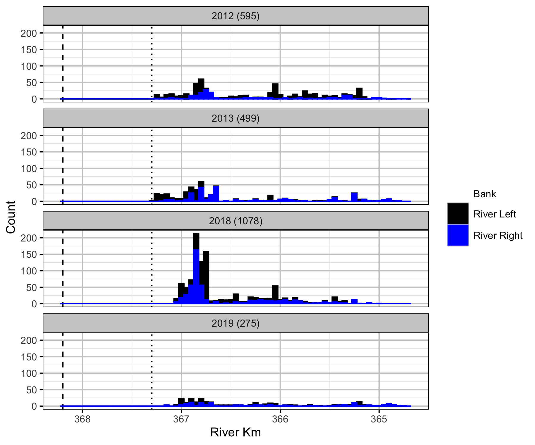
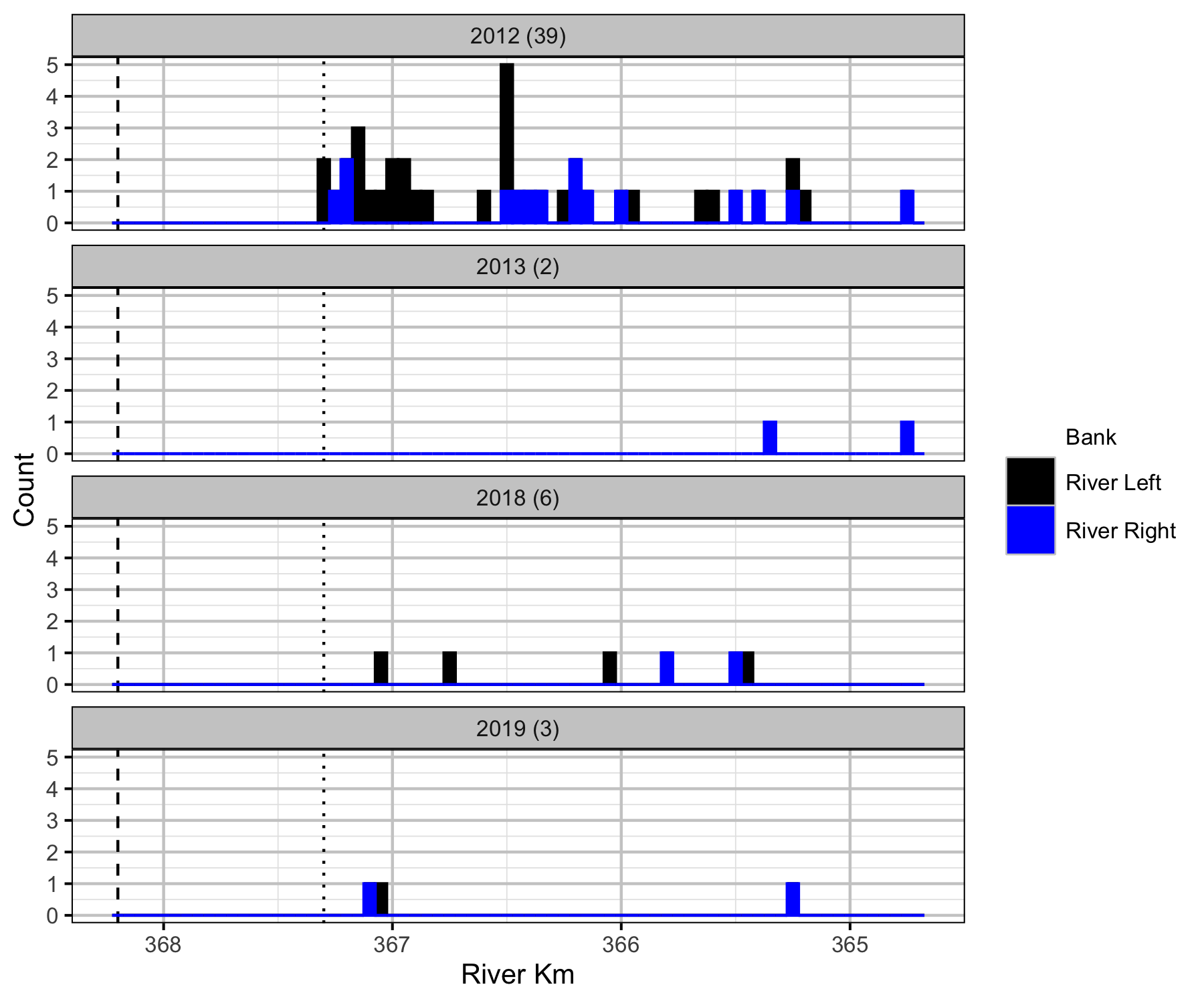
Backpack Electrofishing
Temperature
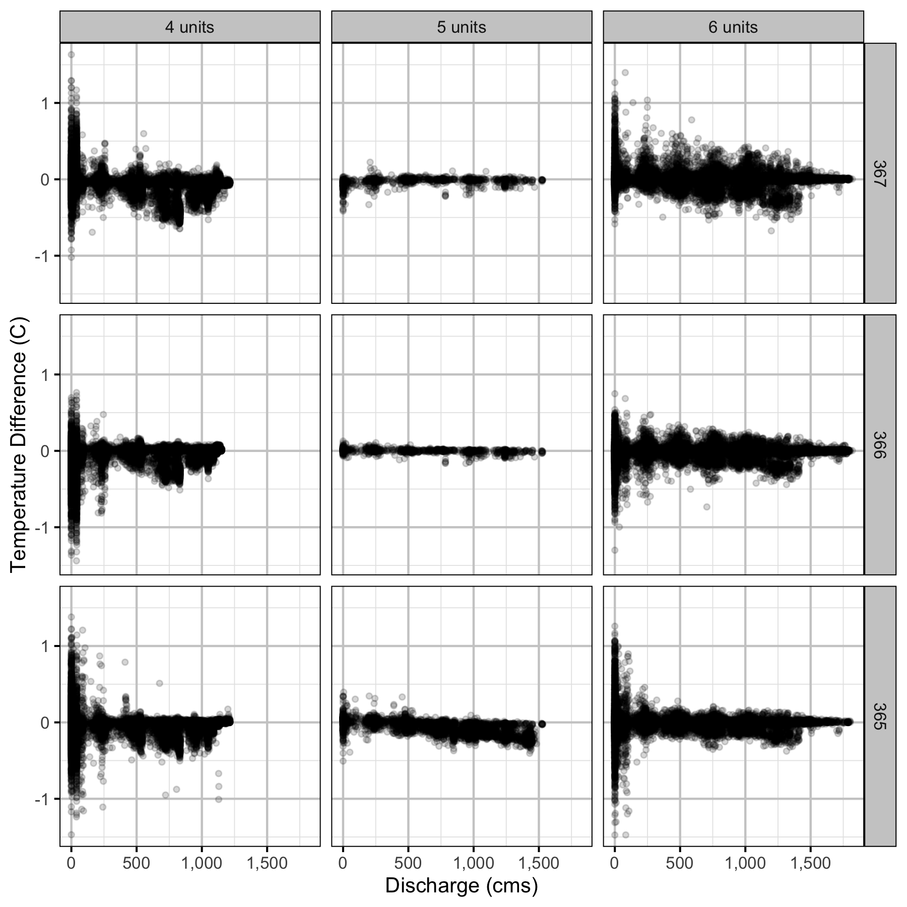
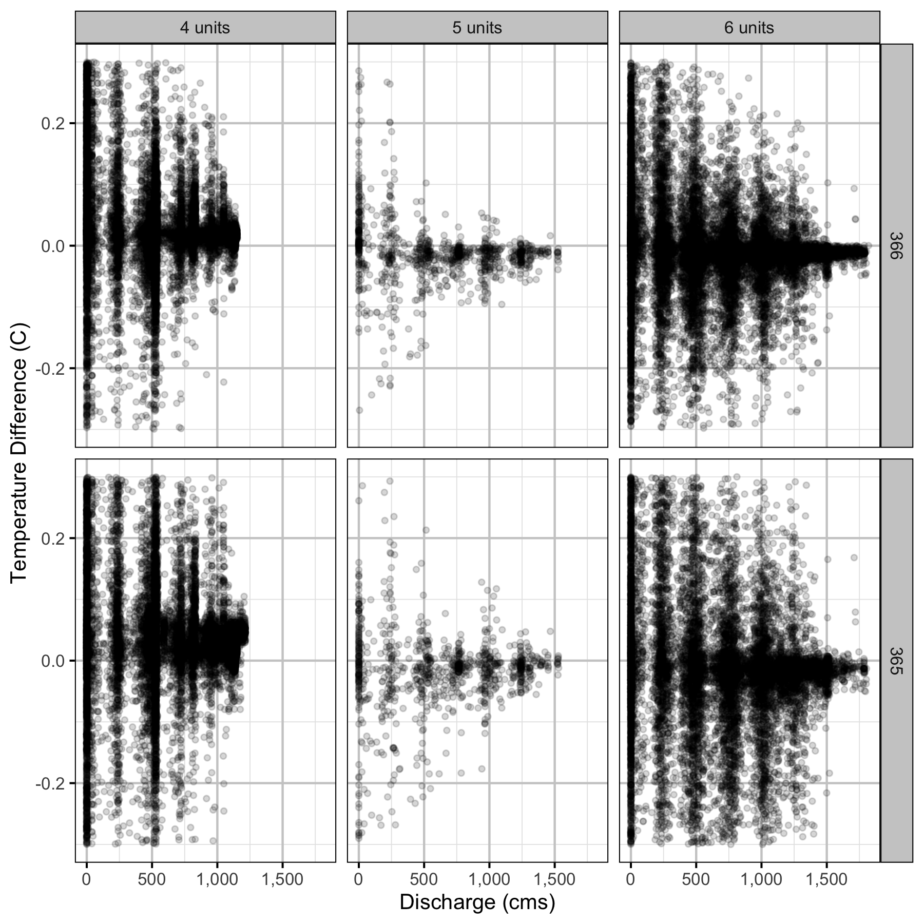
Forebay
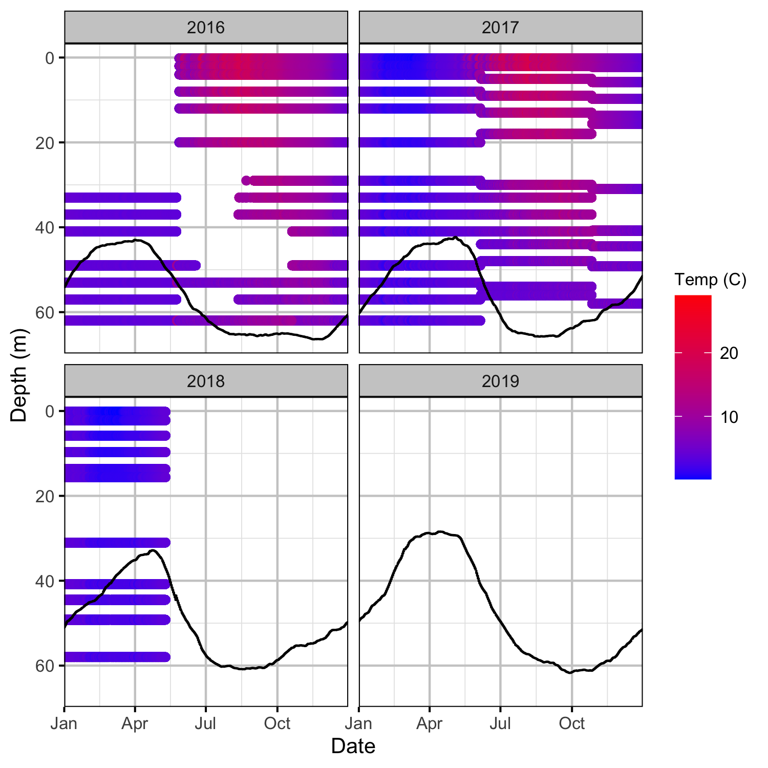
Tailrace
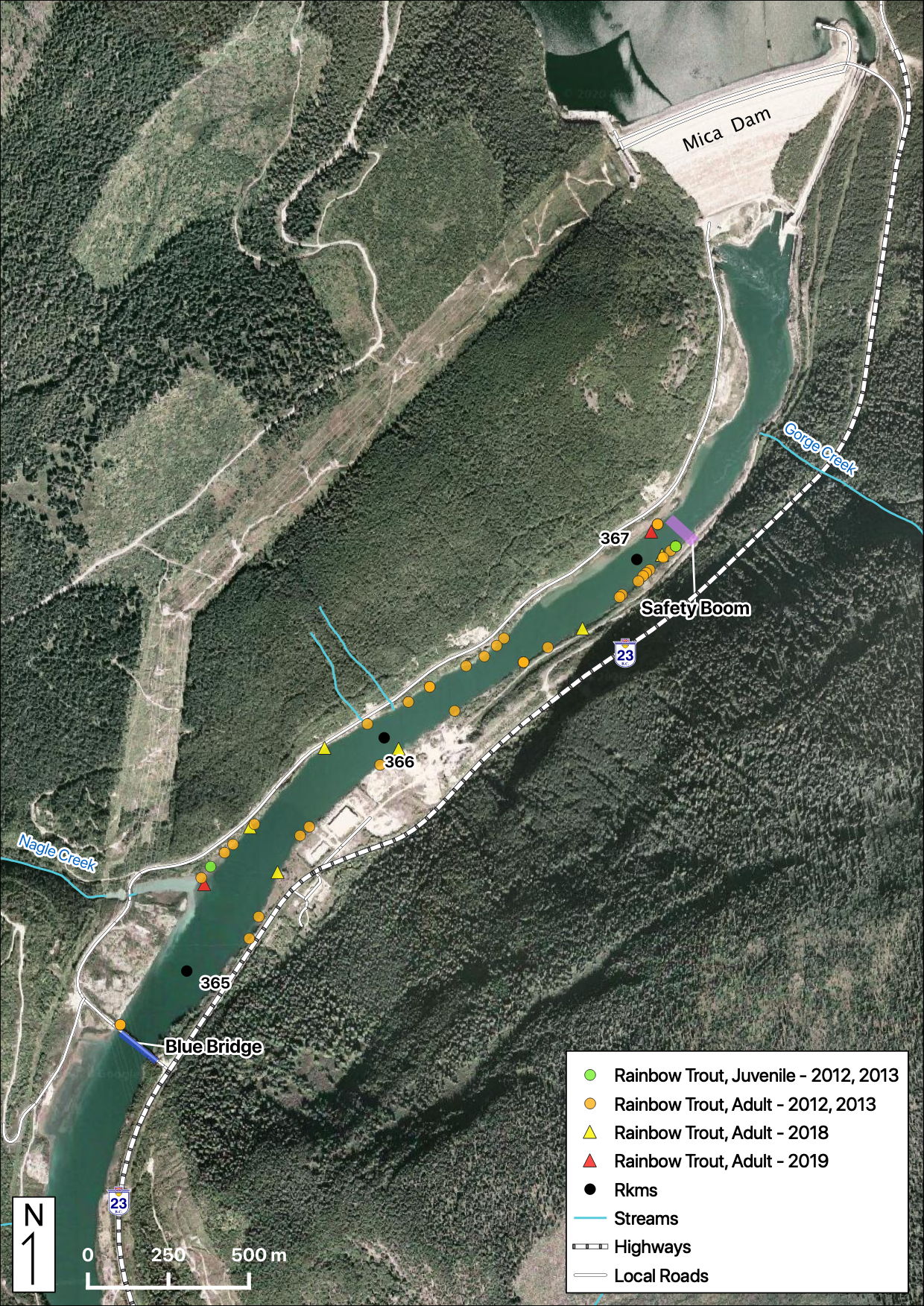
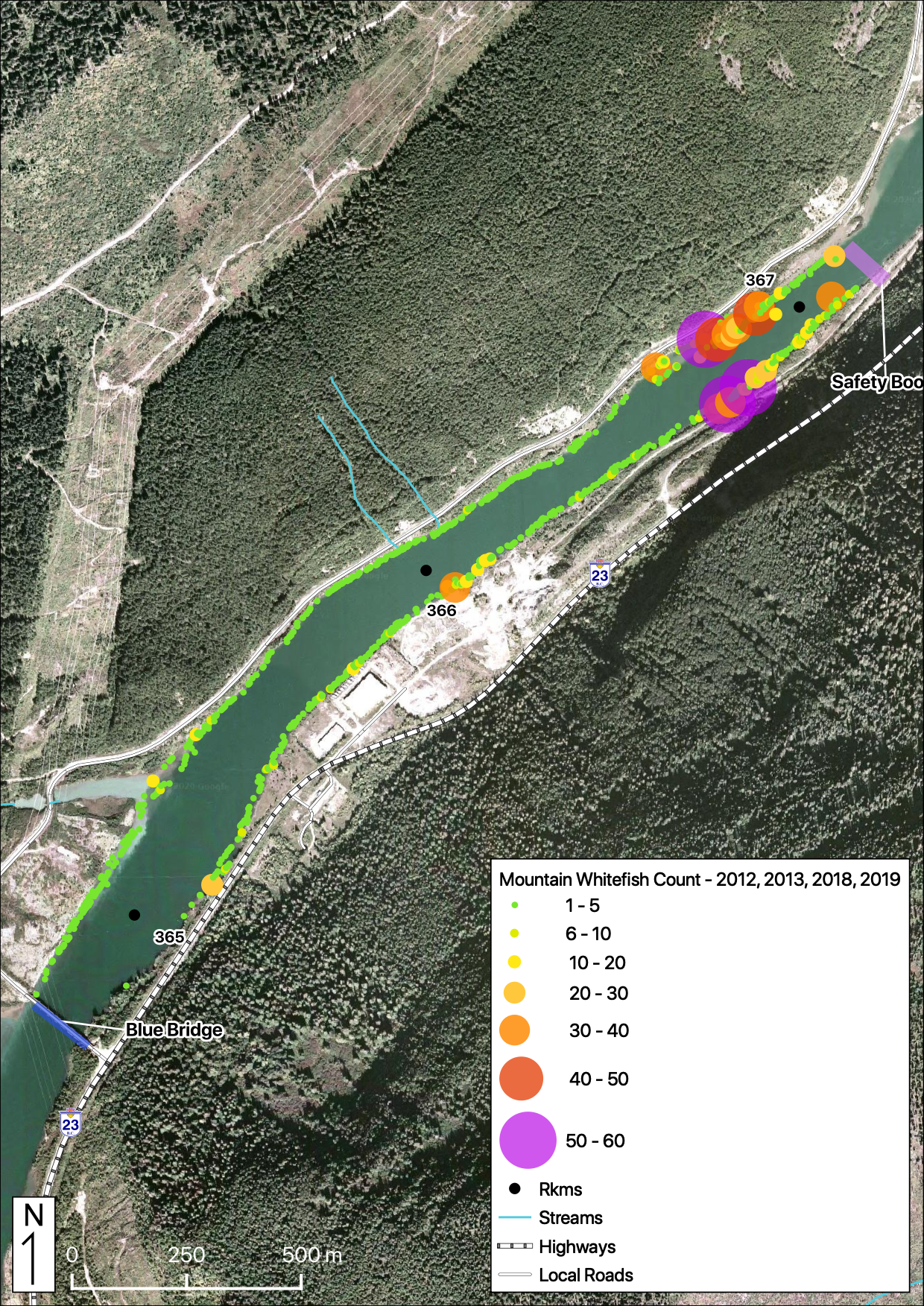
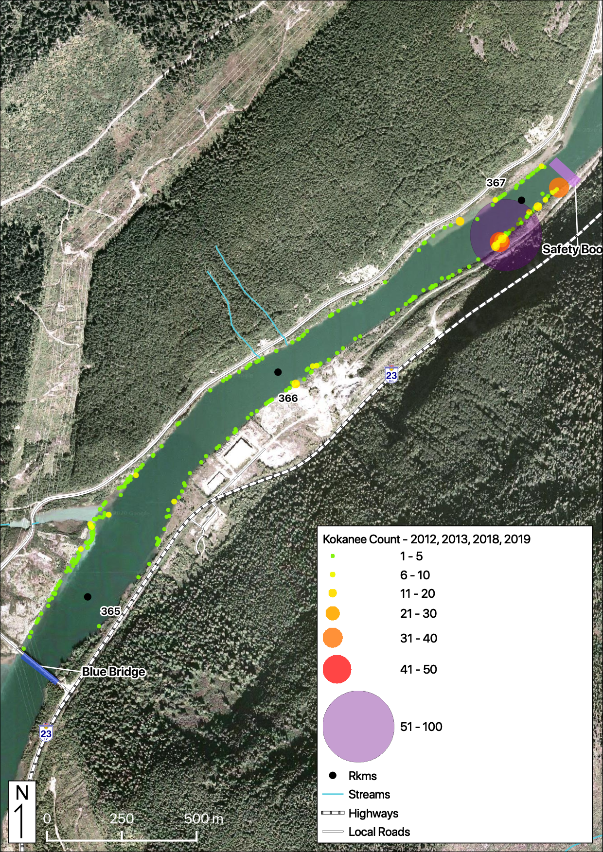
Maps
Sites
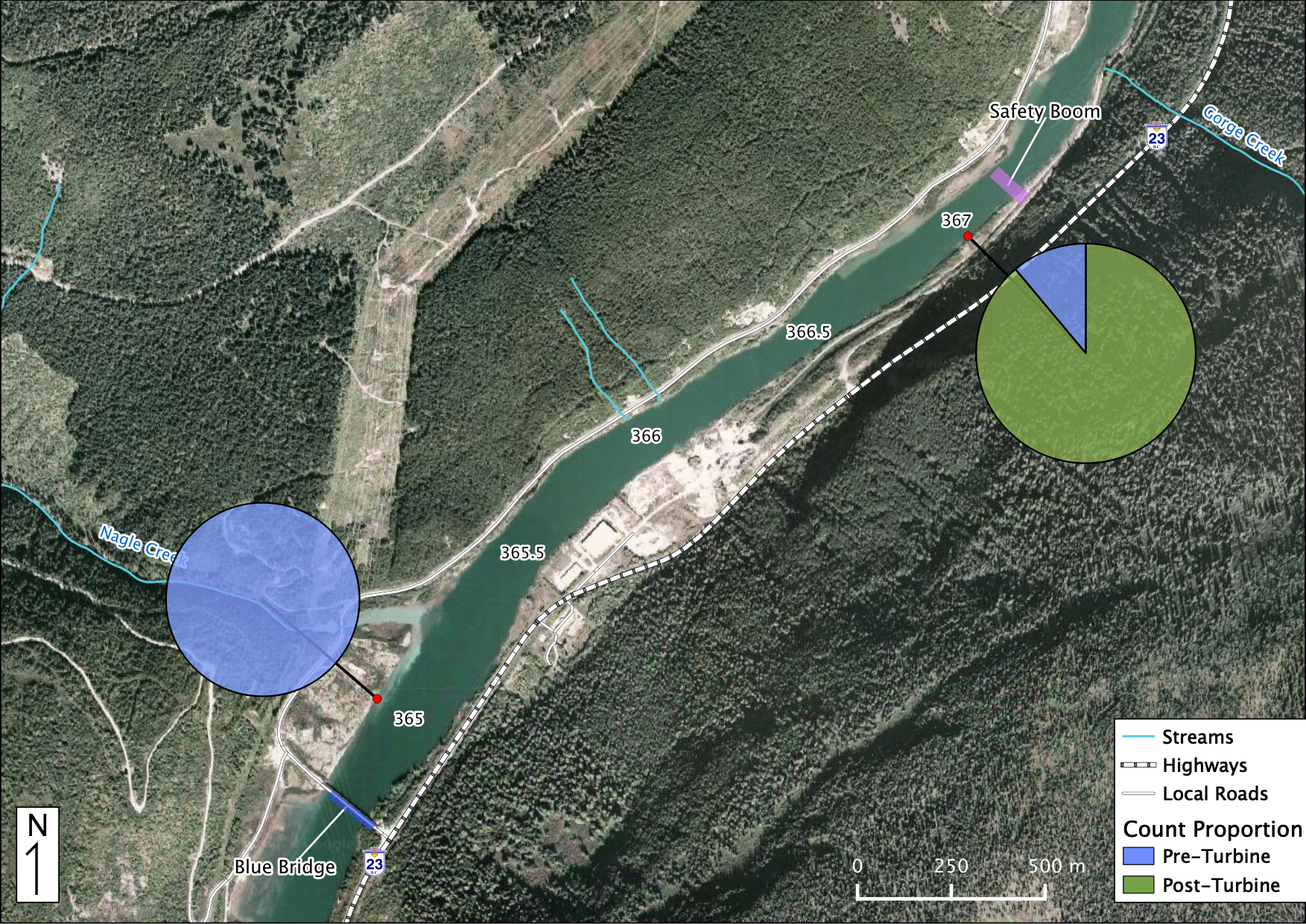
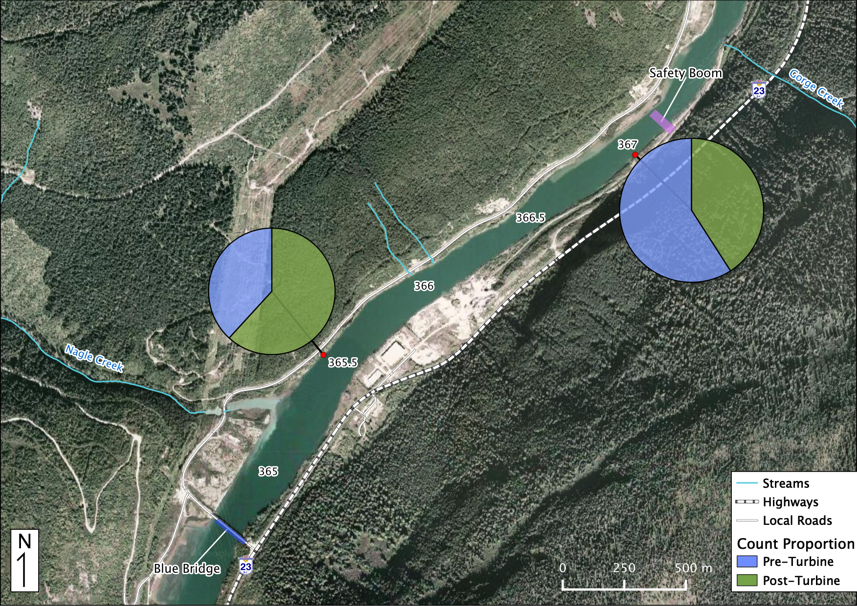
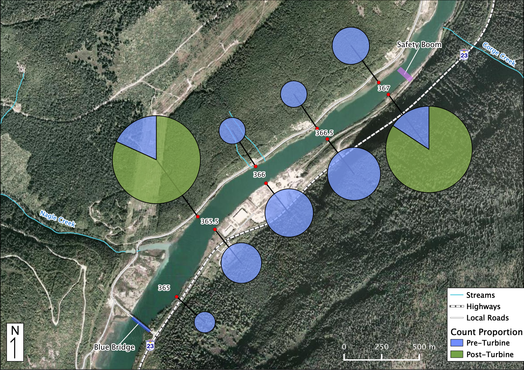
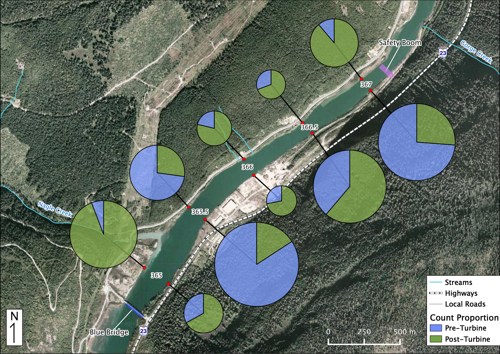
Relative Counts
Total Counts

Acknowledgements
The organisations and individuals whose contributions have made this report possible include:
- BC Hydro
- Trish Joyce
- Jason Watson
- Margo Sadler
- Guy Martel
- Peter McCann
- Fred Katunar
- Alf Leake
- Karen Bray
- Ktunaxa Nation
- Katrina Caley
- Joanne Fisher
- Jim Clarricoates
- Jon Bisset
- Will Warnock
- Bill Green
- Poisson Consulting
- Robyn Irvine
- Seb Dalgarno
- Applied Aquatic Research
- Tom Boag
- Ministry of Forests, Lands and Natural Resource Operations
- Albert Chirico
- Mark Thomas
- Charlotte Houston
References
Bradford, Michael J, Josh Korman, and Paul S Higgins. 2005. “Using Confidence Intervals to Estimate the Response of Salmon Populations (Oncorhynchus Spp.) to Experimental Habitat Alterations.” Canadian Journal of Fisheries and Aquatic Sciences 62 (12): 2716–26. https://doi.org/10.1139/f05-179.
Brooks, Steve, Andrew Gelman, Galin L. Jones, and Xiao-Li Meng, eds. 2011. Handbook for Markov Chain Monte Carlo. Boca Raton: Taylor & Francis.
He, Ji X., James R. Bence, James E. Johnson, David F. Clapp, and Mark P. Ebener. 2008. “Modeling Variation in Mass-Length Relations and Condition Indices of Lake Trout and Chinook Salmon in Lake Huron: A Hierarchical Bayesian Approach.” Transactions of the American Fisheries Society 137 (3): 801–17. https://doi.org/10.1577/T07-012.1.
Kery, Marc, and Michael Schaub. 2011. Bayesian Population Analysis Using WinBUGS : A Hierarchical Perspective. Boston: Academic Press. http://www.vogelwarte.ch/bpa.html.
McElreath, Richard. 2016. Statistical Rethinking: A Bayesian Course with Examples in R and Stan. Chapman & Hall/CRC Texts in Statistical Science Series 122. Boca Raton: CRC Press/Taylor & Francis Group.
Plummer, Martyn. 2015. “JAGS Version 4.0.1 User Manual.” http://sourceforge.net/projects/mcmc-jags/files/Manuals/4.x/.
R Core Team. 2015. “R: A Language and Environment for Statistical Computing.” Vienna, Austria: R Foundation for Statistical Computing. http://www.R-project.org/.
———. 2018. R: A Language and Environment for Statistical Computing. Vienna, Austria: R Foundation for Statistical Computing. https://www.R-project.org/.