Middle Columbia River Fish Indexing Analysis 2017
The suggested citation for this analytic report is:
Thorley, J.L. (2018) Middle Columbia River Fish Indexing Analysis 2017. A Poisson Consulting Analysis Report. URL: https://www.poissonconsulting.ca/f/77904731.
Background
The key management questions to be addressed by the analyses are:
- Is there a change in abundance of adult life stages of fish using the Middle Columbia River (MCR) that corresponds with the implementation of a year-round minimum flow?
- Is there a change in growth rate of adult life stages of the most common fish species using the MCR that corresponds with the implementation of a year-round minimum flow?
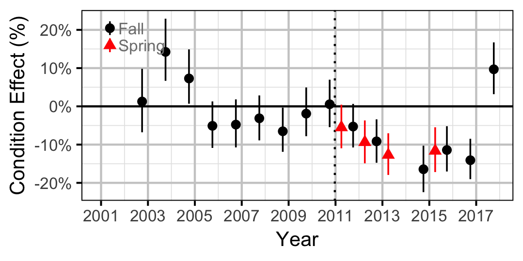
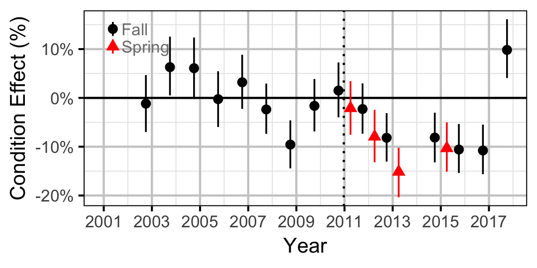
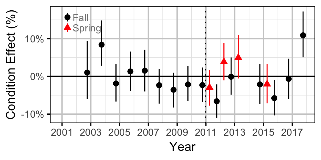
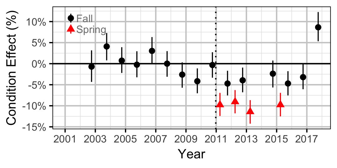
- Is there a change in body condition (measured as a function of relative weight to length) of adult life stages of fish using the MCR that corresponds with the implementation of a year-round minimum flow?
- Is there a change in spatial distribution of adult life stages of fish using the MCR that corresponds with the implementation of a year-round minimum flow?
Other objectives include the estimation of species richness, species diversity (evenness) and the modeling of environmental-fish metric relationships and scale age data. The year-round minimum flow was implemented in the winter of 2010 at the same time that a fifth turbine was added.
Methods
Data Preparation
The data were collected by Okanagan Nation Alliance and Golder Associates.
Life-Stage
The four primary fish species were categorized as fry, juvenile or adult based on their lengths.
Table 1. Length cutoffs by species and stage.
| Species | Fry | Juvenile |
|---|---|---|
| Bull Trout | < 120 | < 400 |
| Mountain Whitefish | < 120 | < 175 |
| Rainbow Trout | < 120 | < 250 |
| Largescale Sucker | < 120 | < 350 |
Statistical Analysis
Model parameters were estimated using Bayesian methods. The Bayesian estimates were produced using JAGS (Plummer 2015) and STAN (Carpenter et al. 2017). For additional information on Bayesian estimation the reader is referred to McElreath (2016).
Unless indicated otherwise, the Bayesian analyses used uninformative normal prior distributions (Kery and Schaub 2011, 36). The posterior distributions were estimated from 1500 Markov Chain Monte Carlo (MCMC) samples thinned from the second halves of 3 chains (Kery and Schaub 2011, 38–40). Model convergence was confirmed by ensuring that \(\hat{R} \leq 1.1\) (Kery and Schaub 2011, 40) and \(\textrm{ESS} \geq 150\) for each of the monitored parameters (Kery and Schaub 2011, 61). Where \(\hat{R}\) is the potential scale reduction factor and \(\textrm{ESS}\) is the effective sample size.
The parameters are summarised in terms of the point estimate, standard deviation (sd), the z-score, lower and upper 95% confidence/credible limits (CLs) and the p-value (Kery and Schaub 2011, 37, 42). For Bayesian models, the estimate is the median (50th percentile) of the MCMC samples, the z-score is \(\mathrm{mean}/\mathrm{sd}\) and the 95% CLs are the 2.5th and 97.5th percentiles. A p-value of 0.05 indicates that the lower or upper 95% CL is 0.
Where relevant, model adequacy was confirmed by examination of residual plots.
The results are displayed graphically by plotting the modeled relationships between particular variables and the response(s) with the remaining variables held constant. In general, continuous and discrete fixed variables are held constant at their mean and first level values, respectively, while random variables are held constant at their typical values (expected values of the underlying hyperdistributions) (Kery and Schaub 2011, 77–82). When informative the influence of particular variables is expressed in terms of the effect size (i.e., percent change in the response variable) with 95% confidence/credible intervals (CIs, Bradford, Korman, and Higgins 2005).
The analyses were implemented using R version 3.5.0
(R Core Team 2015) and the
mbr family of packages.
Growth
Annual growth was estimated from the inter-annual recaptures using the Fabens method (Fabens 1965) for estimating the von Bertalanffy (VB) growth curve (von Bertalanffy 1938). The VB curves is based on the premise that
\[ \frac{dl}{dt} = k (L_{\infty} - l)\]
where \(l\) is the length of the individual, \(k\) is the growth coefficient and \(L_{\infty}\) is the mean maximum length.
Integrating the above equation gives
\[ l_t = L_{\infty} (1 - e^{-k(t - t0)})\]
where \(l_t\) is the length at time \(t\) and \(t0\) is the time at which the individual would have had no length.
The Fabens form allows
\[ l_r = l_c + (L_{\infty} - l_c) (1 - e^{-kT})\]
where \(l_r\) is the length at recapture, \(l_c\) is the length at capture and \(T\) is the time at large.
Key assumptions of the growth model include:
- \(k\) can vary with discharge regime and randomly with year.
- The residual variation in growth is normally distributed.
Mountain Whitefish with a FL \(>\) 250 mm at release were excluded from the growth analysis as they appeared to be undergoing biphasic growth.
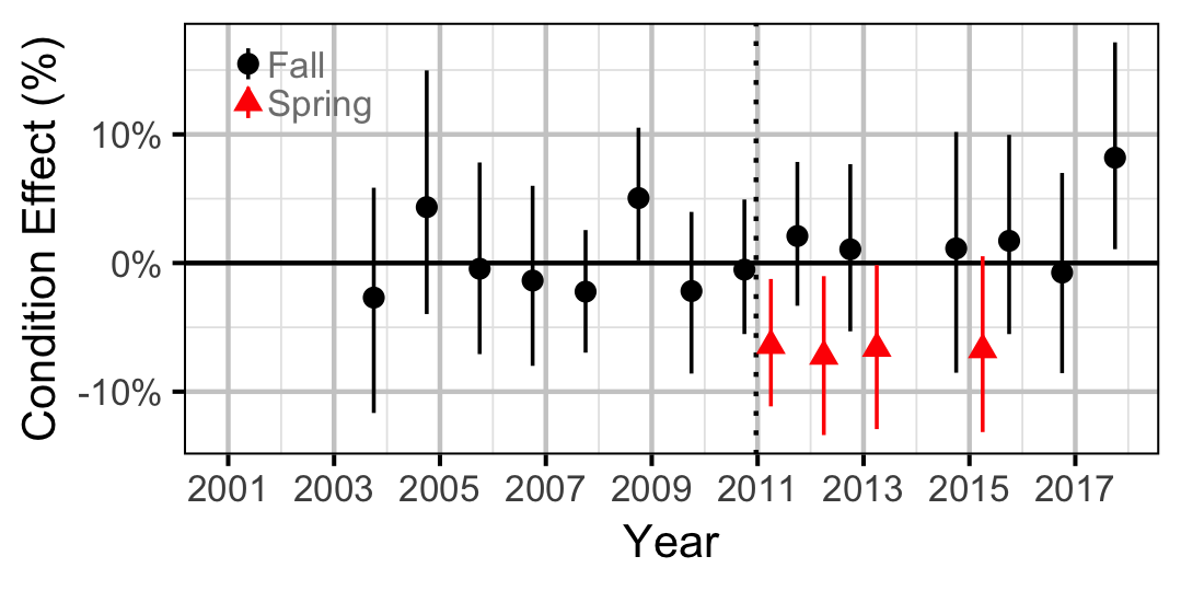
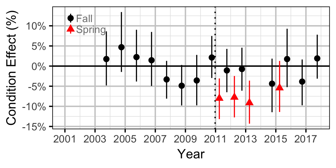
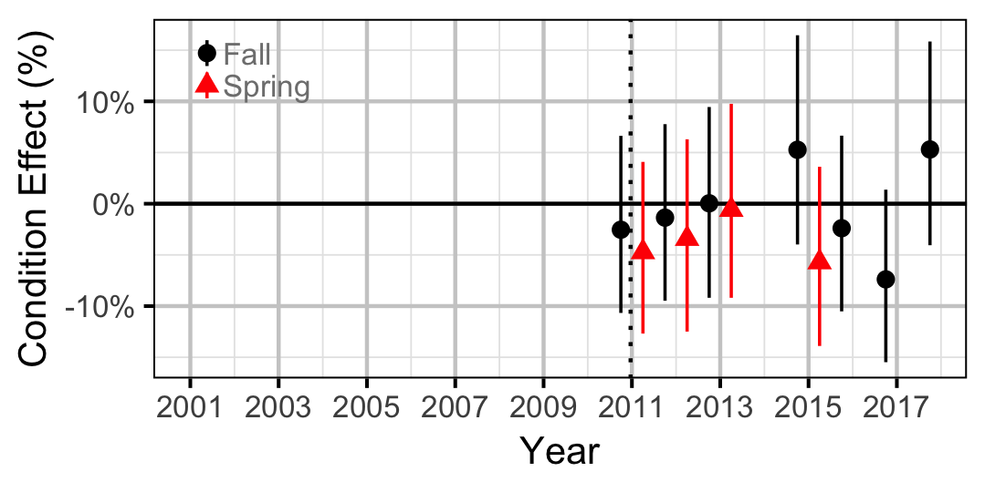
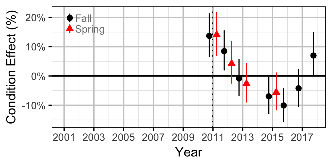
Condition
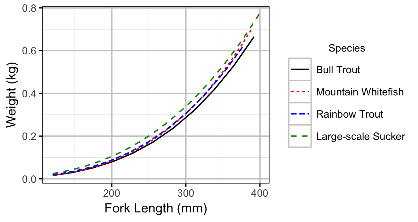
Condition was estimated via an analysis of mass-length relations (He et al. 2008).
More specifically the model was based on the allometric relationship
\[ W = \alpha L^{\beta}\]
where \(W\) is the weight (mass), \(\alpha\) is the coefficent, \(\beta\) is the exponent and \(L\) is the length.
To improve chain mixing the relation was log-transformed, i.e.,
\[ \log(W) = \log(\alpha) + \beta \log(L)\]
and the logged lengths centered, i.e., \(\log(L) - \overline{\log(L)}\), prior to model fitting.
Key assumptions of the condition model include:
- \(\alpha\) can vary with the regime and season and randomly with year.
- \(\beta\) can vary with the regime and season and randomly with year.
- The residual variation in weight is log-normally distributed.
Fry were excluded from the condition analysis.
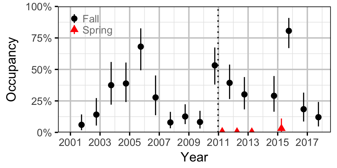
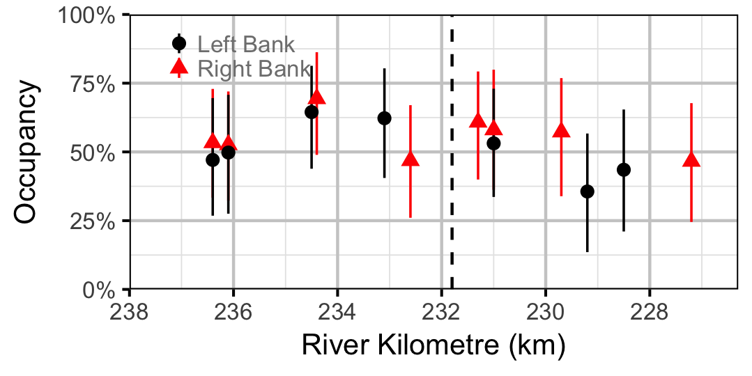
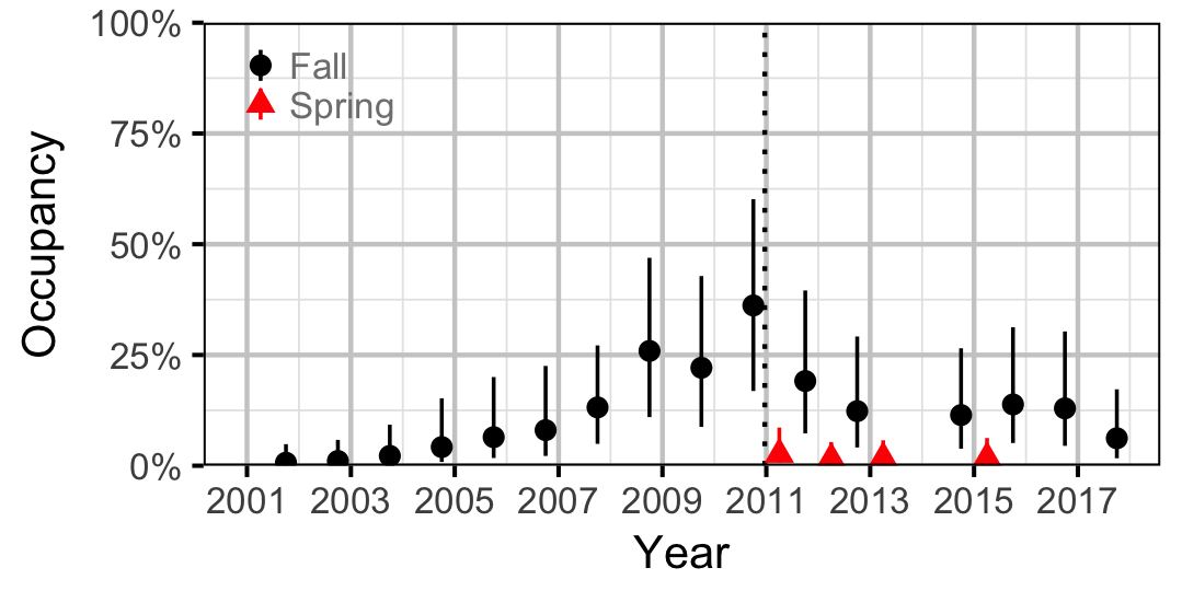
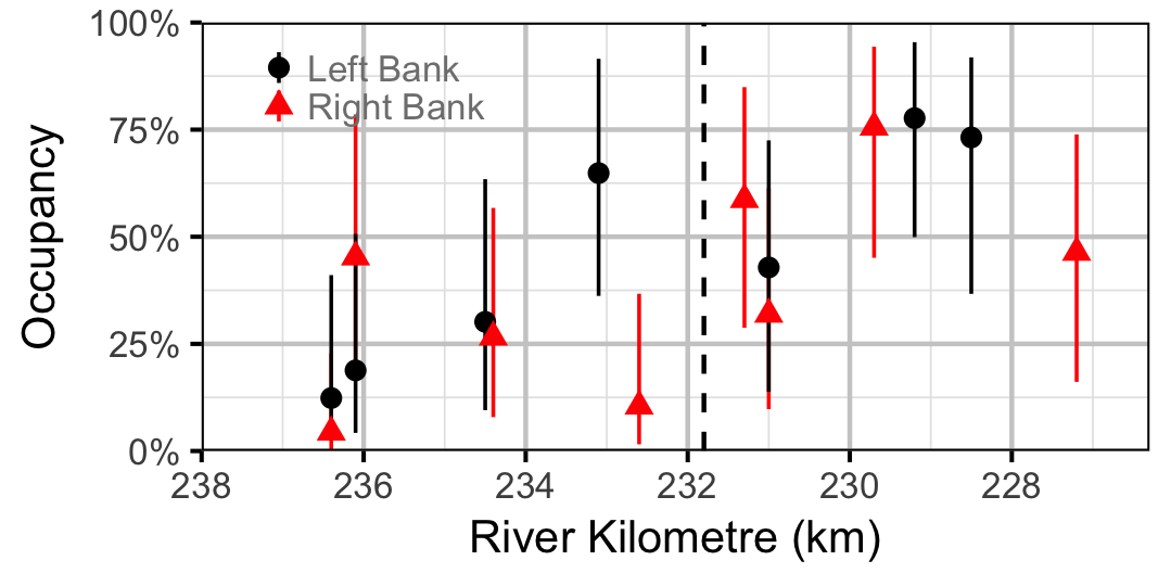
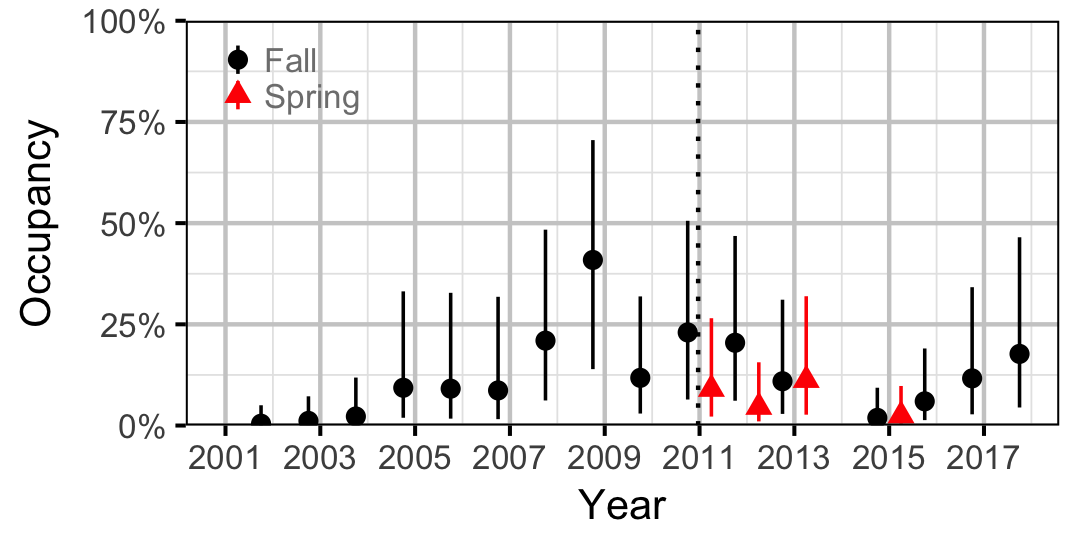
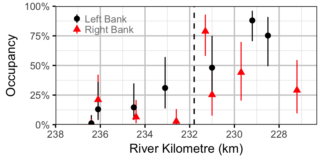
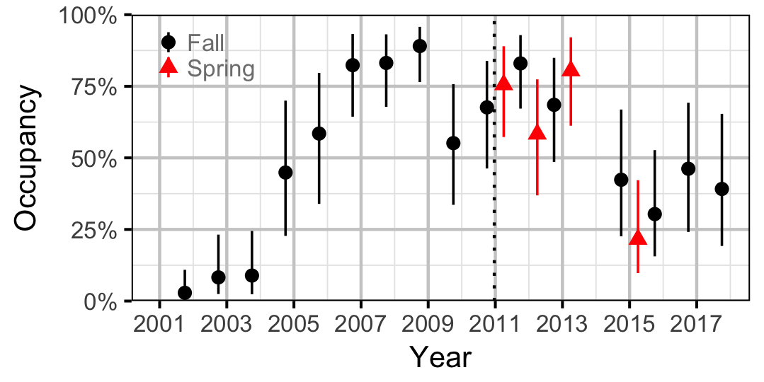
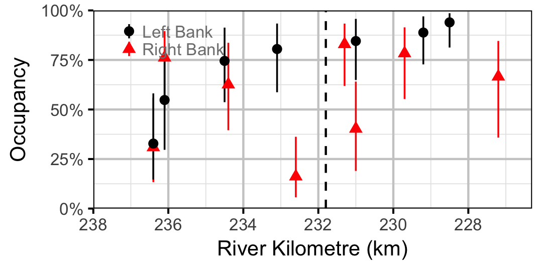
Occupancy
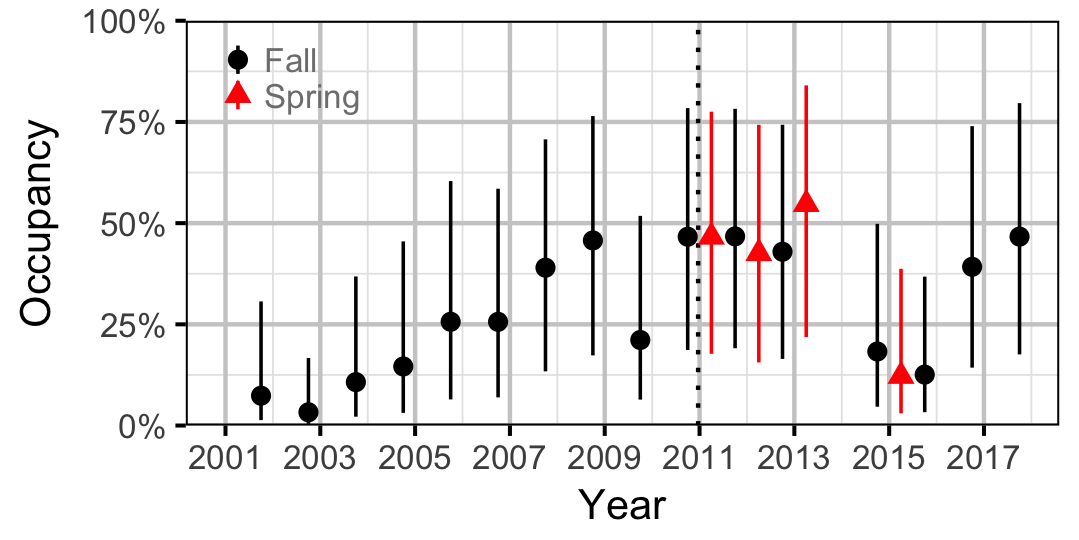
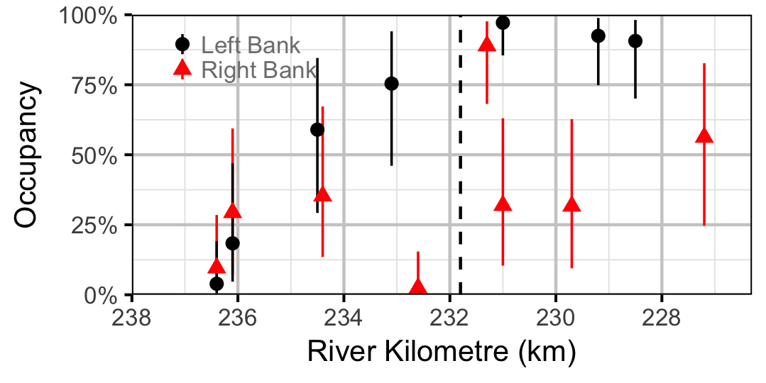
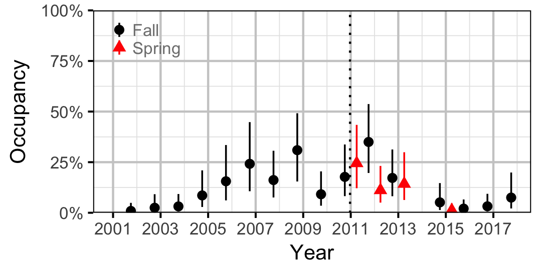
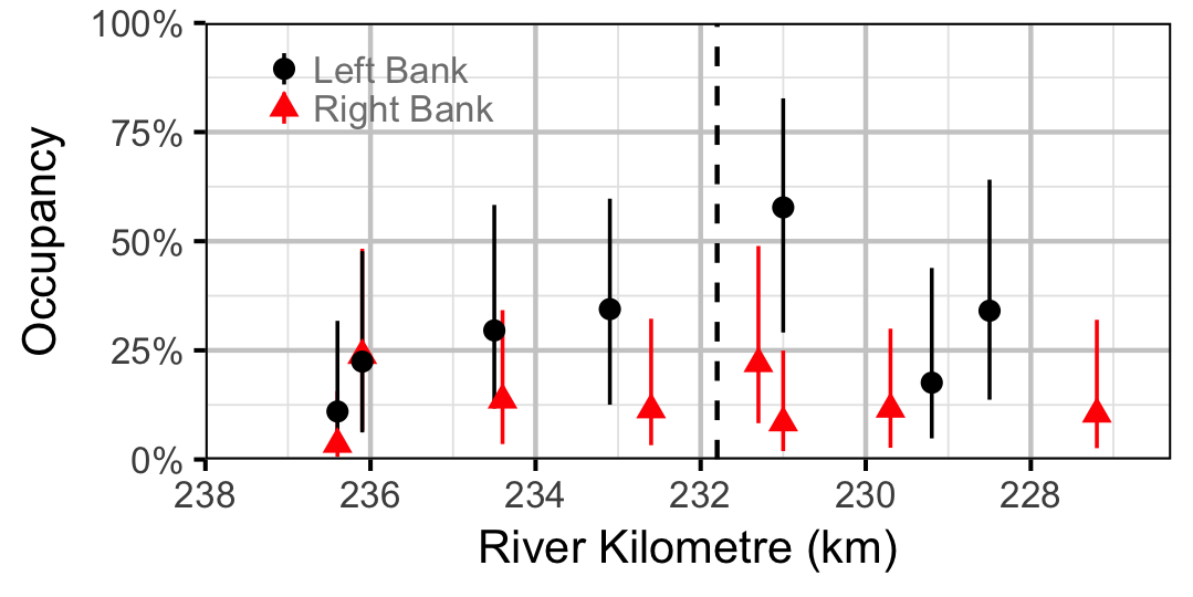
Occupancy, which is the probability that a particular species was present at a site, was estimated from the temporal replication of detection data (Kery and Schaub 2011, 414–18), i.e., each site was surveyed multiple times within a season. A species was considered to have been detected if one or more individuals of the species were caught or counted. It is important to note that the model estimates the probability that the species was present at a given (or typical) site in a given (or typical) year as opposed to the probability that the species was present in the entire study area. We focused on Northern Pikeminnow, Burbot, Lake Whitefish, Rainbow Trout, Redside Shiner and Sculpins because they were low enough density to not to be present at all sites at all times yet were encounted sufficiently often to provide information on spatial and temporal changes.
Key assumptions of the occupancy model include:
- Occupancy varies with season.
- Occupancy varies randomly with site and site within year.
- The effect of year on occupancy is autoregressive with a lag of one year and varies with discharge regime.
- Sites are closed, i.e., the species is present or absent at a site for all the sessions in a particular season of a year.
- Observed presence is described by a bernoulli distribution, given occupancy.
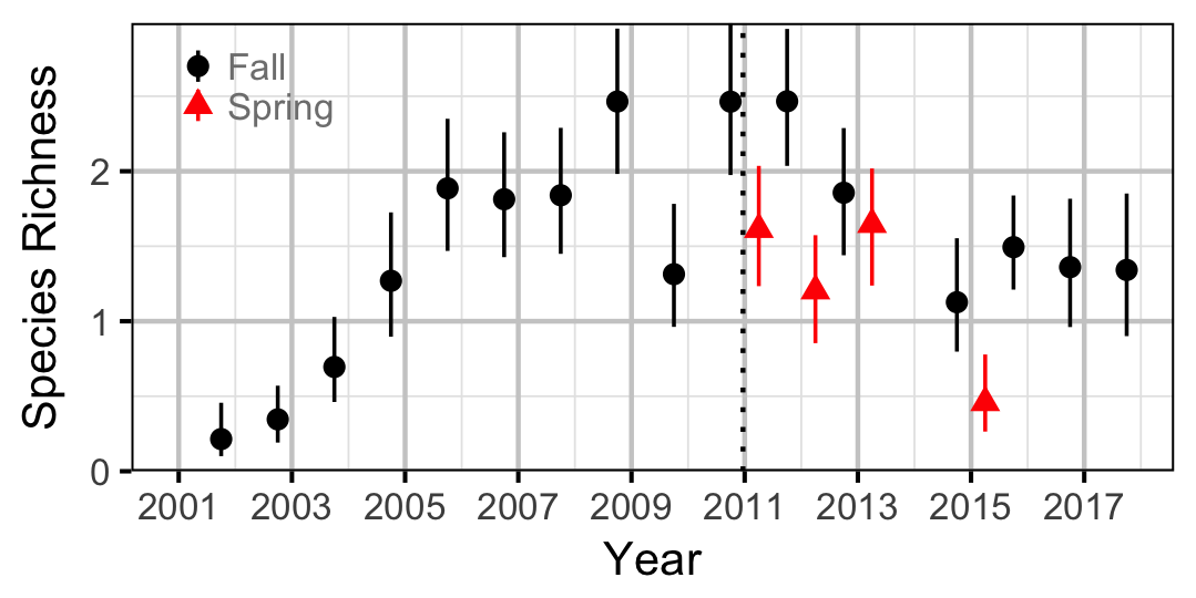
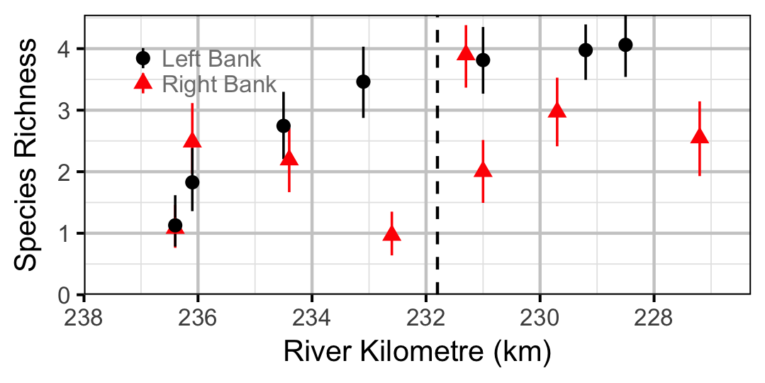
Species Richness
The estimated probabilities of presence for the six species considered in the occupany analyses were summed to give the expected species richnesses by site and year.
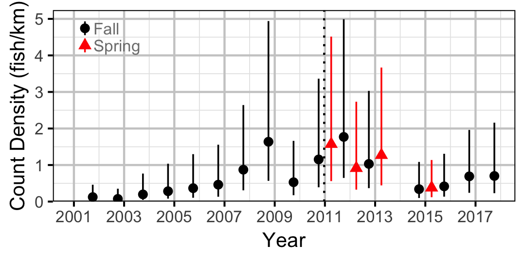
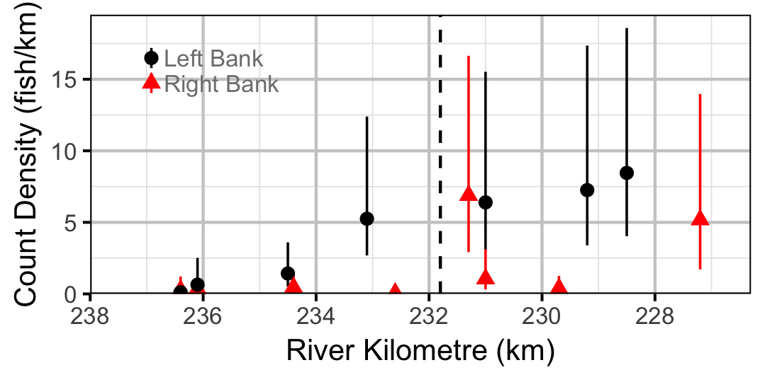
Count
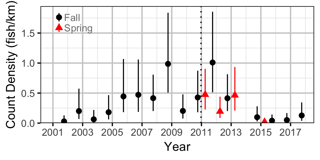
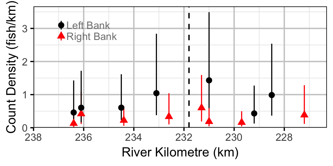
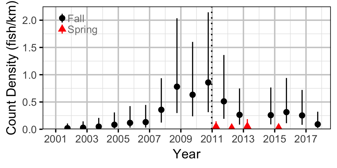
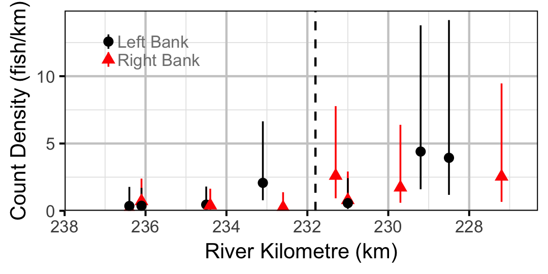
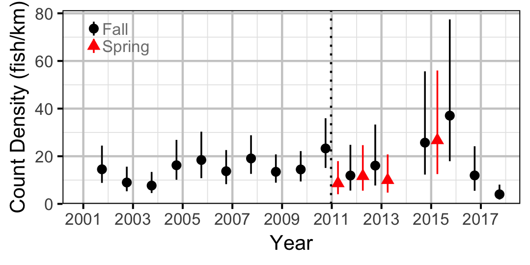
The count data were analysed using an overdispersed Poisson model (Kery 2010, pp 168-170; Kery and Schaub 2011, pp 55-56) to provide estimates of the lineal river count density (count/km). The model estimates the expected count which is the product of the abundance and observer efficiency. In order to interpret the estimates as relative densities it is necessary to assume that changes in observer efficiency are negligible.
Key assumptions of the count model include:
- The count density (count/km) varies as an exponential growth model with the rate of change varying with discharge regime.
- The count density varies with season.
- The count density varies randomly with site, year and site within year.
- The counts are gamma-Poisson distributed.
In the case of suckers the count model replaced the first assumption with
- The count density varies with discharge regime.
Movement
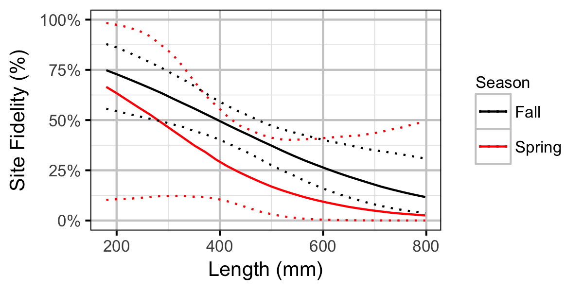
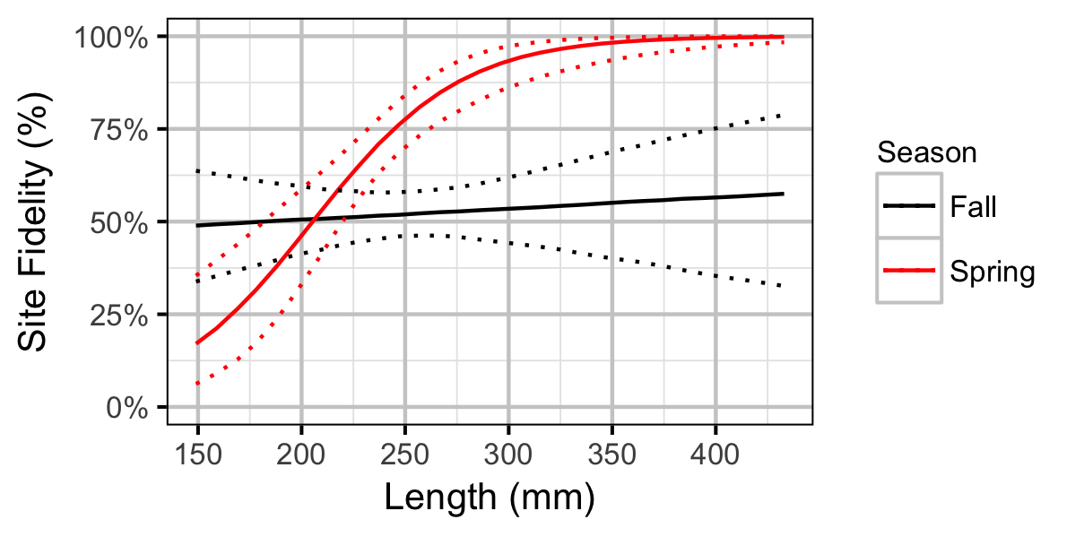
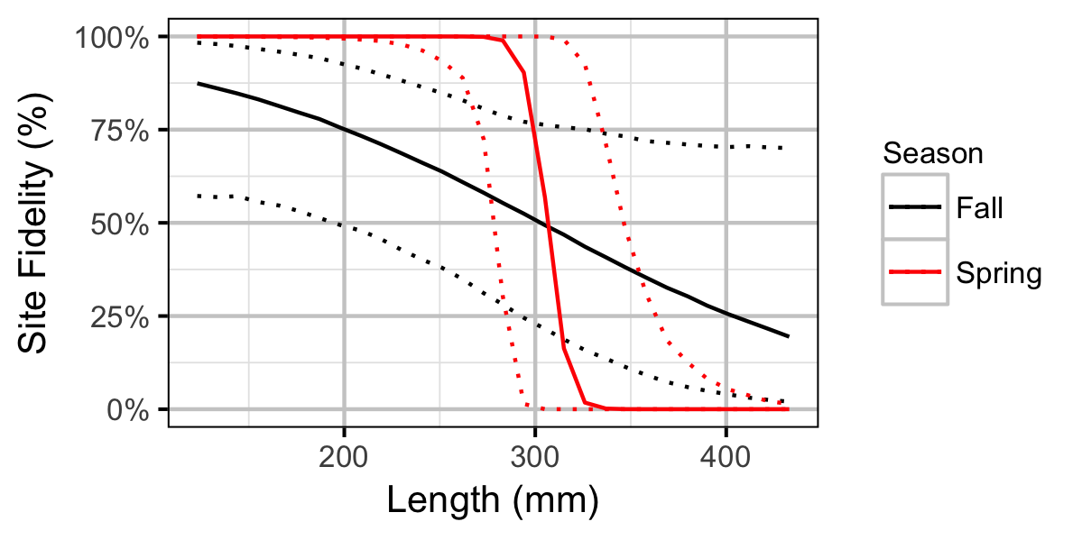
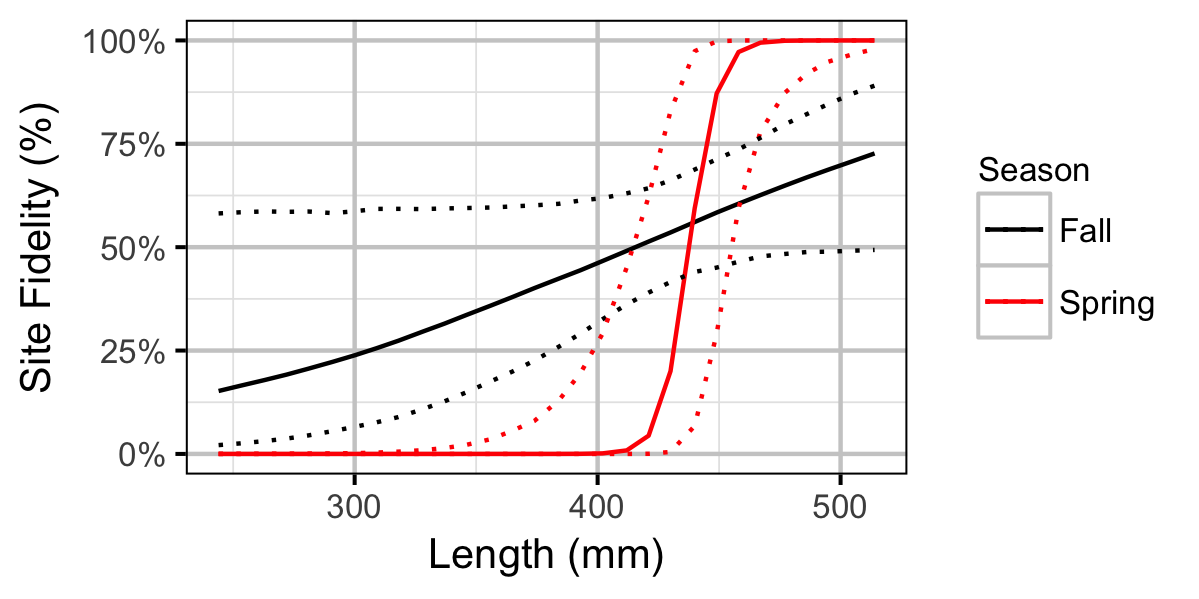
The extent to which sites are closed, i.e., fish remain at the same site between sessions, was evaluated from a logistic ANCOVA (Kery 2010). The model estimated the probability that intra-annual recaptures were caught at the same site versus a different one.
Key assumptions of the site fidelity model include:
- Site fidelity varies with season, fish length and the interaction between season and fish length.
- Observed site fidelity is Bernoulli distributed.
Fry were excluded from the movement analysis.
Observer Length Correction
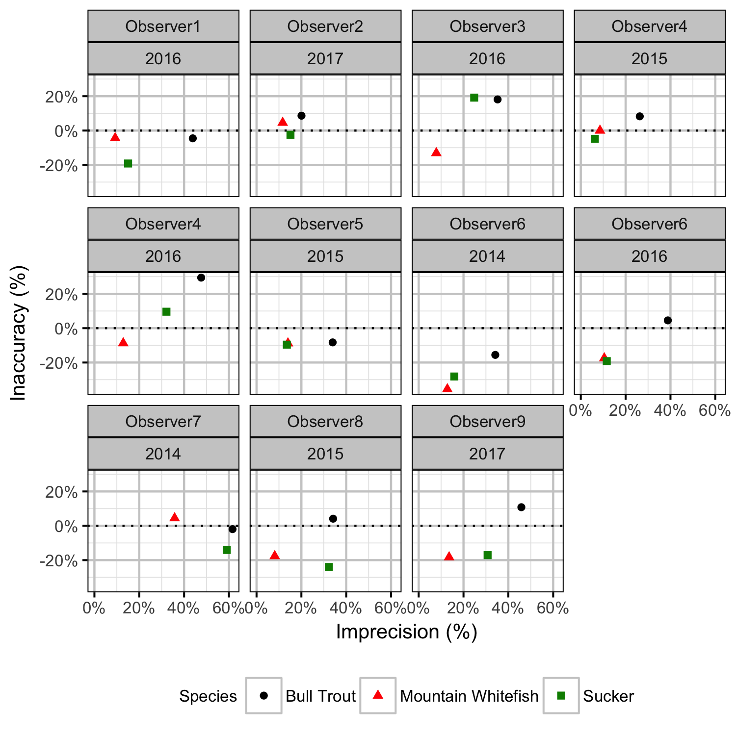
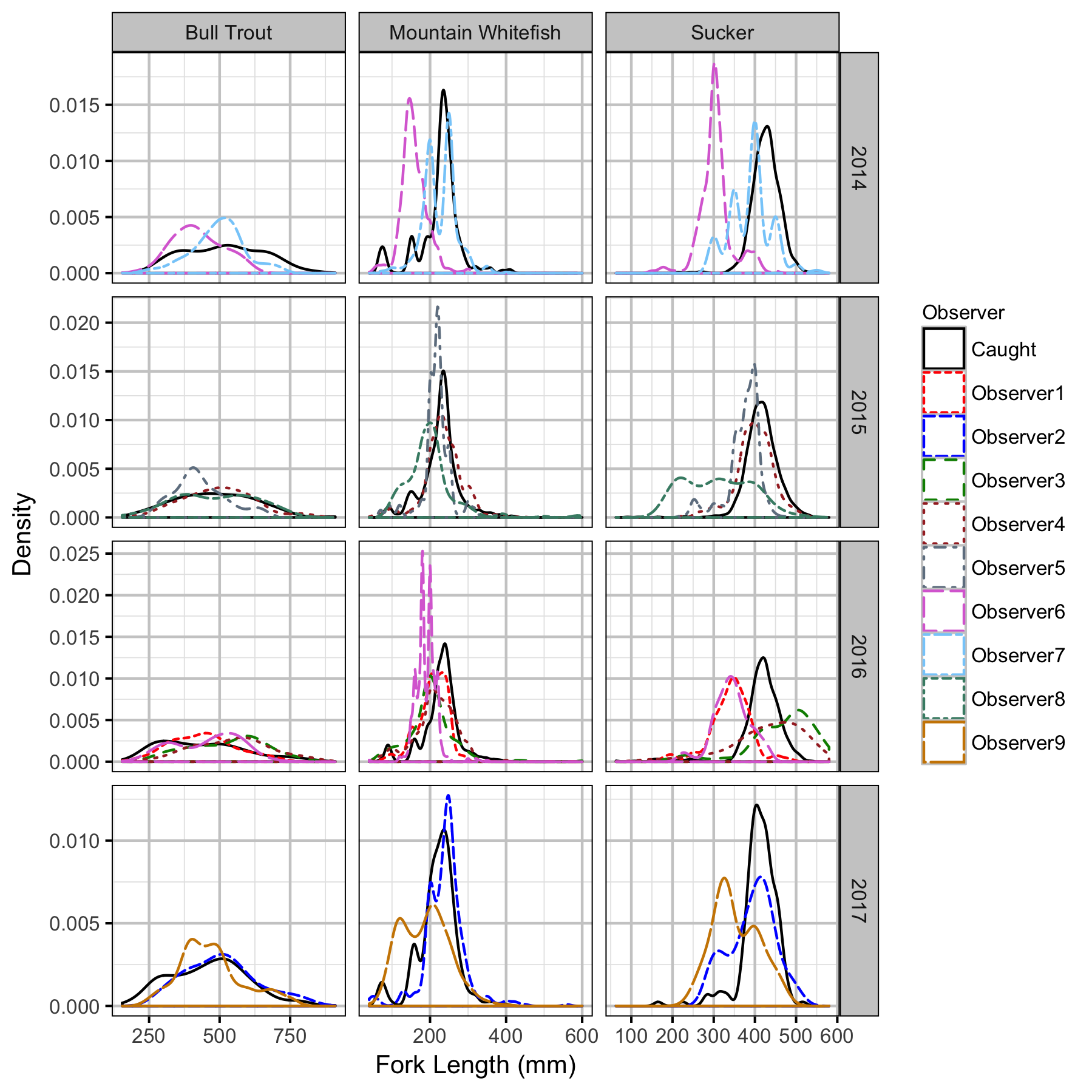
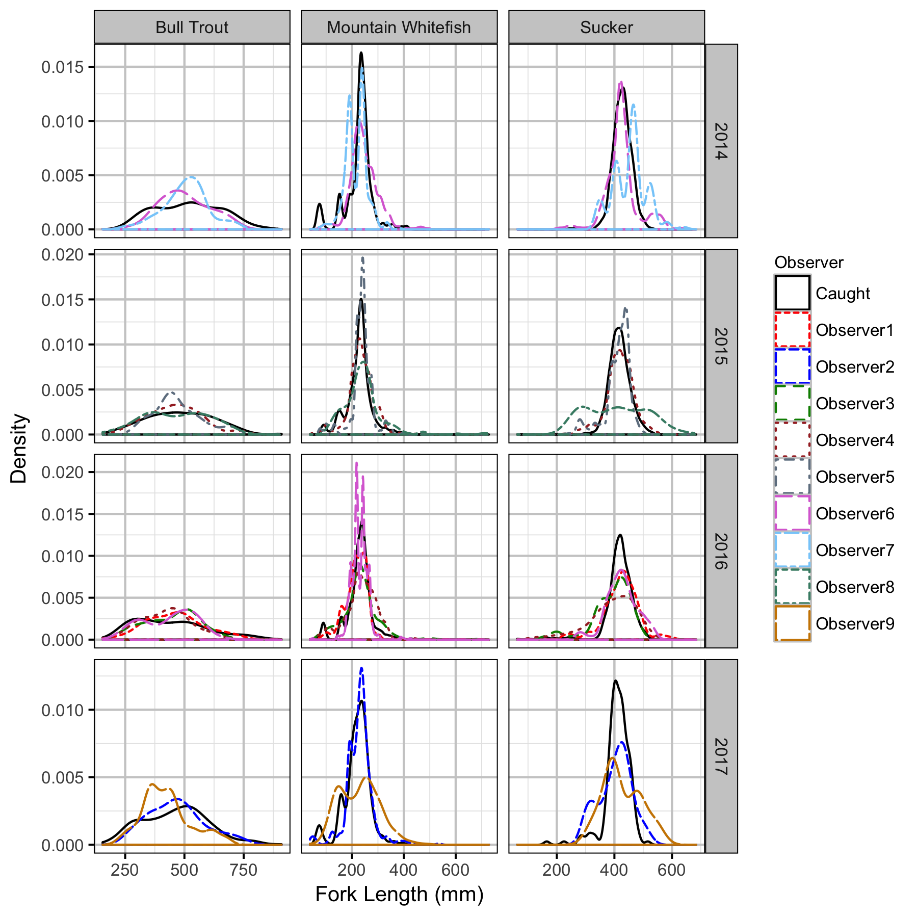
The annual bias (inaccuracy) and error (imprecision) in observer’s fish length estimates were quantified from the divergence of the length distribution of their observed fish from the length distribution of the measured fish. More specifically, the percent length correction that minimised the Jensen-Shannon divergence (Lin 1991) between the two distributions provided a measure of the inaccuracy while the minimum divergence (the Jensen-Shannon divergence was calculated with log to base 2 which means it lies between 0 and 1) provided a measure of the imprecision.
Abundance
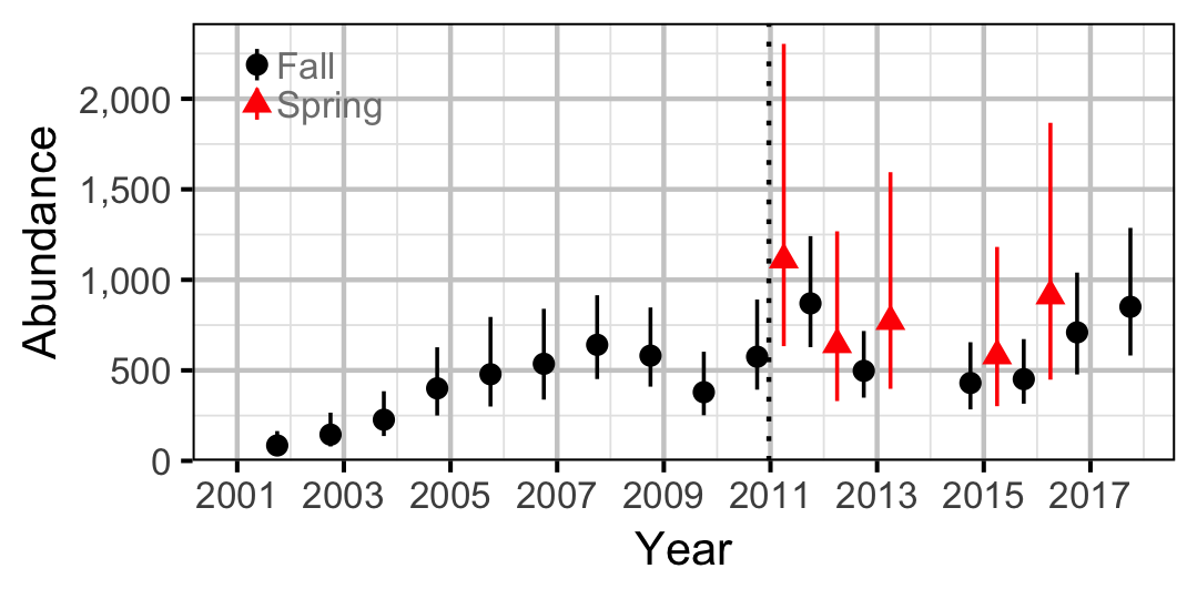
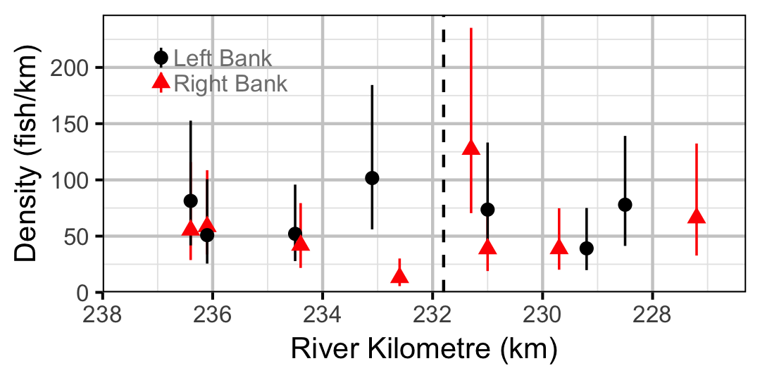
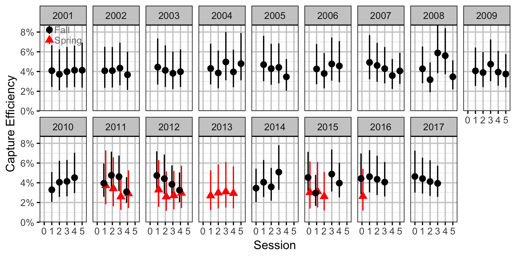
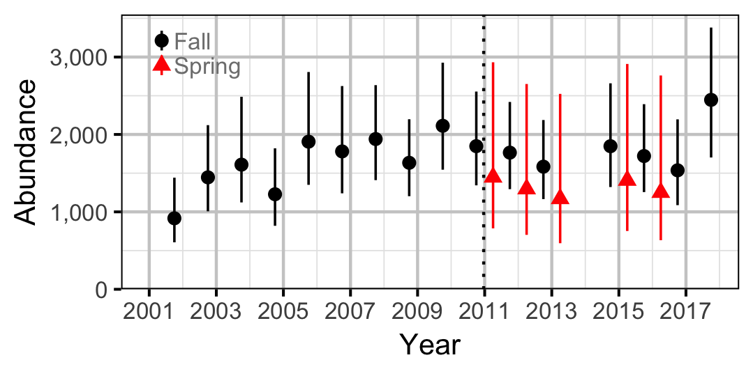
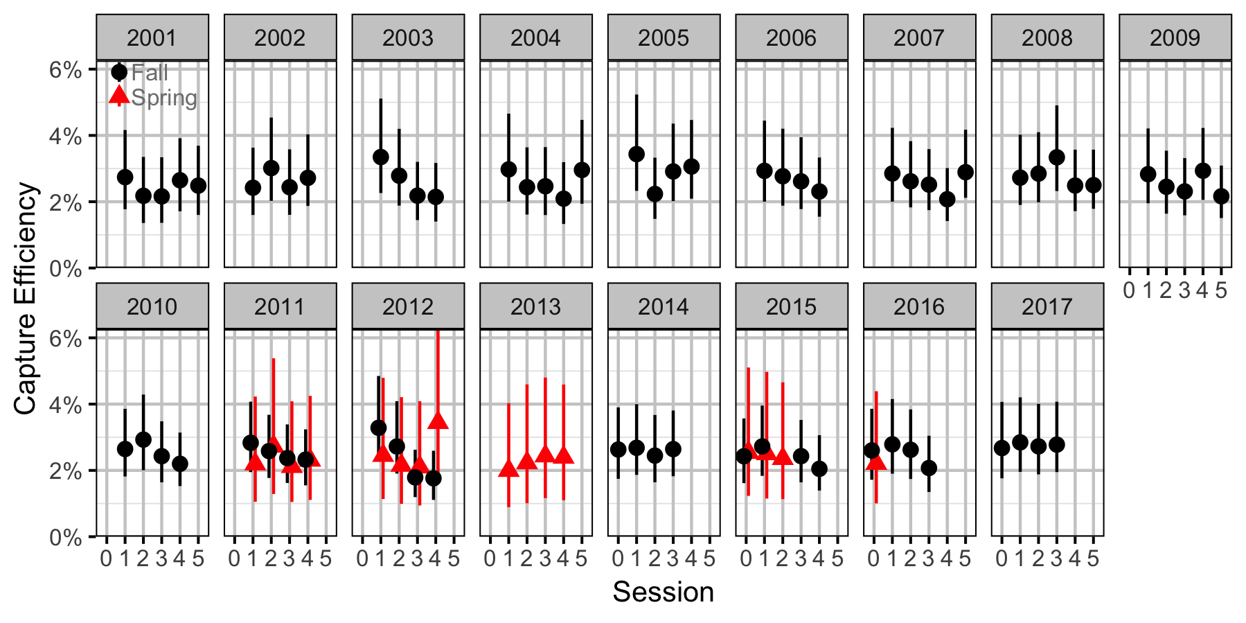
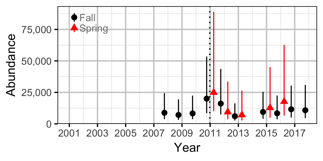
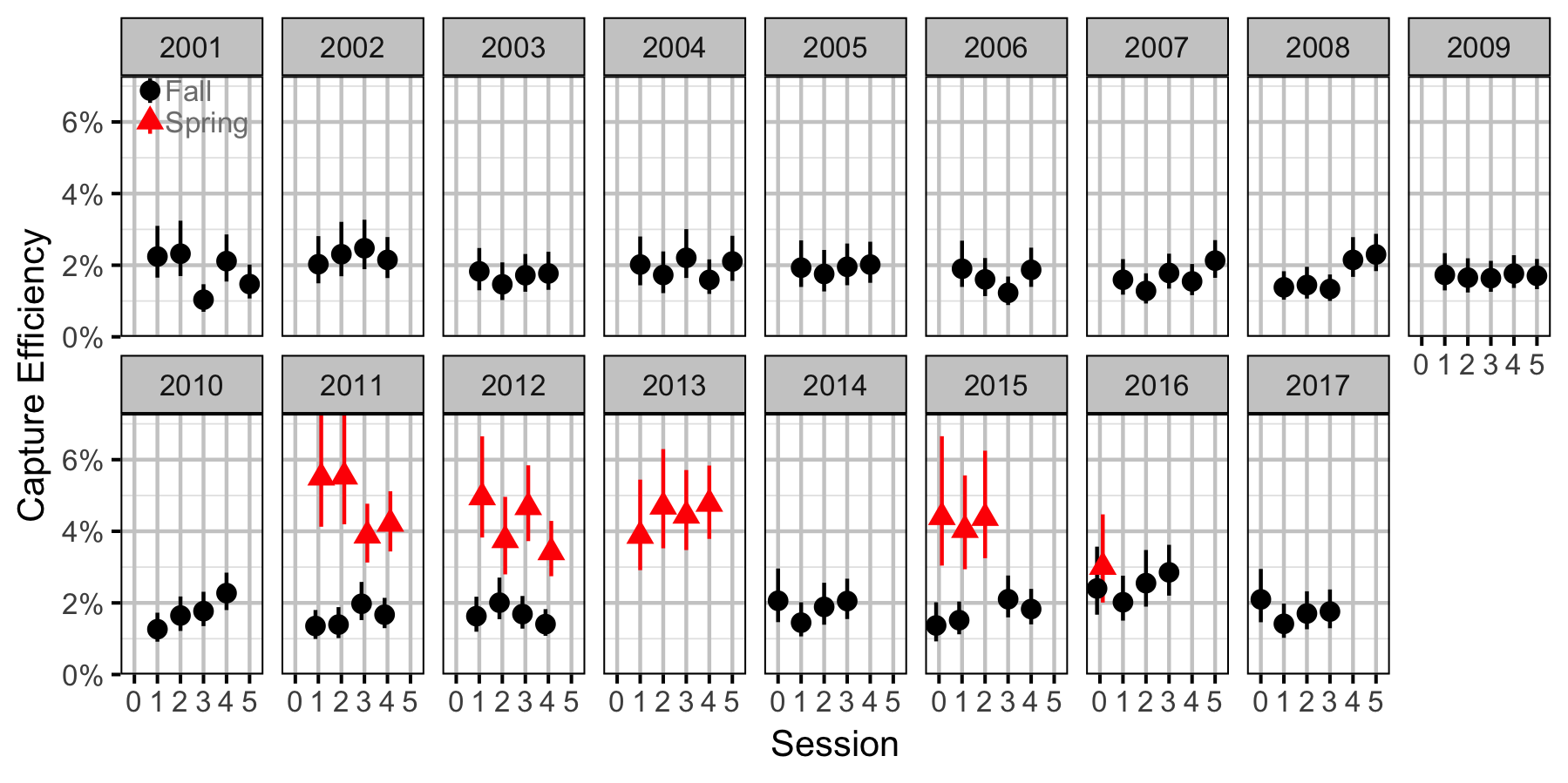
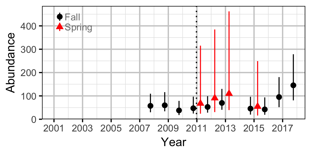
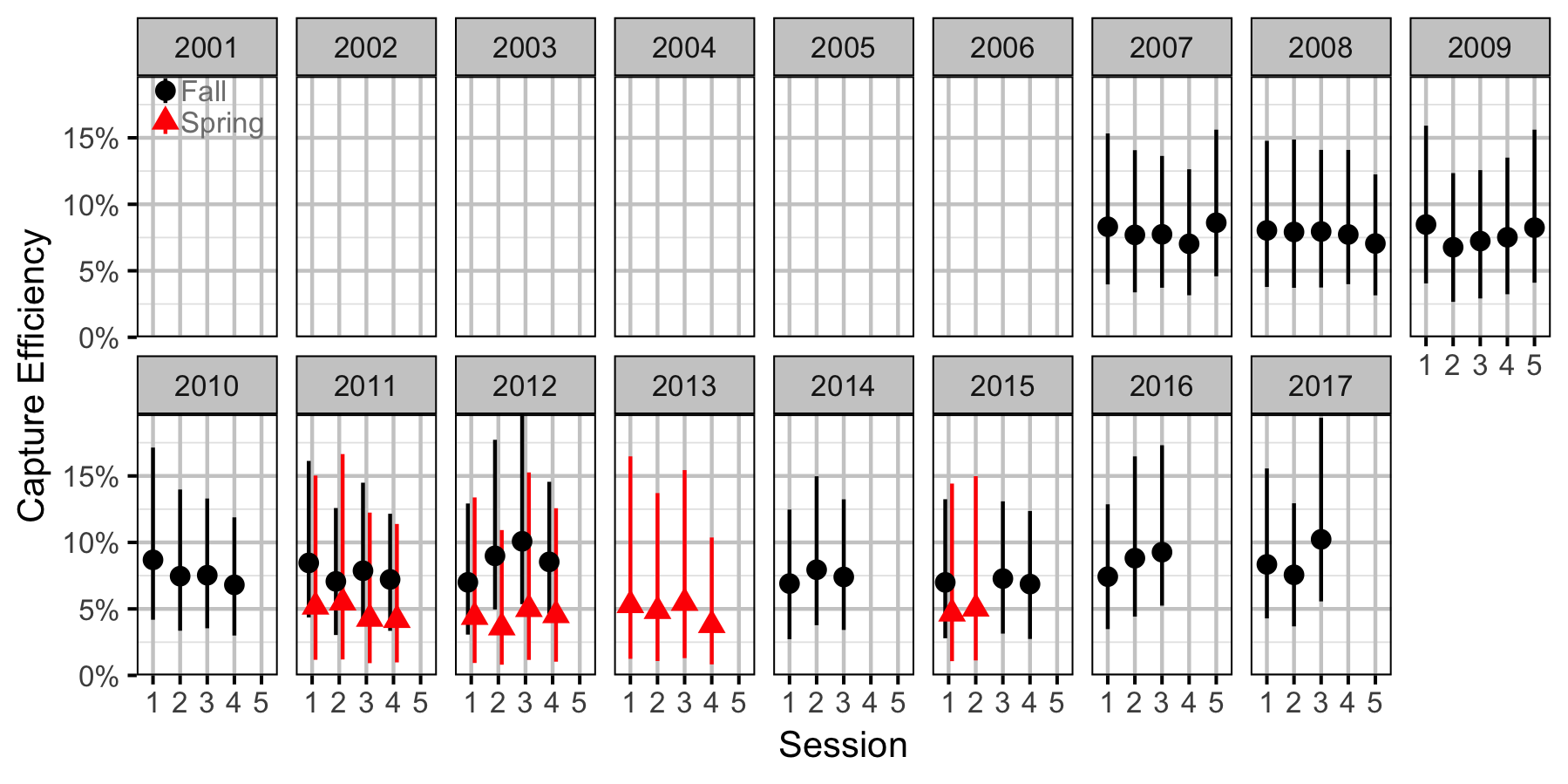
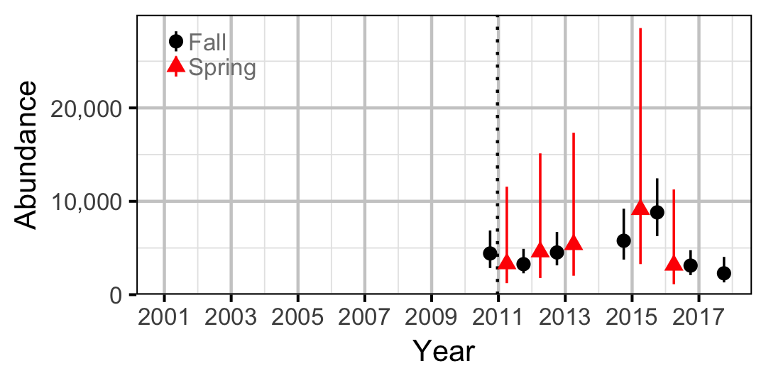
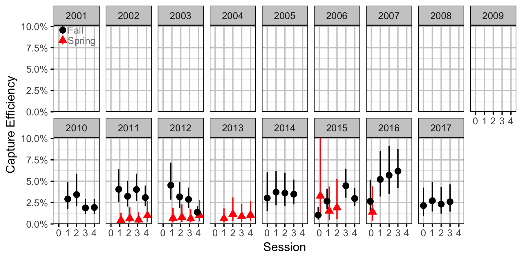
The catch and geo-referenced count data were analysed using a capture-recapture-based overdispersed gamma-Poisson model to provide estimates of capture efficiency and absolute abundance. To maximize the number of recaptures the model grouped all the sites into a supersite for the purposes of estimating the number of marked fish but analysed the total captures at the site level.
Key assumptions of the full abundance model include:
- The density (fish/km) varies as an exponential growth model with the rate of change varying with discharge regime.
- The density varies with season.
- The density varies randomly with site, year and site within year.
- Efficiency (probability of capture) varies by season and method (capture versus count).
- Efficiency varies randomly by session within season within year.
- Marked and unmarked fish have the same probability of capture.
- There is no tag loss, migration (at the supersite level), mortality or misidentification of fish.
- The number of fish caught is gamma-Poisson distributed.
- The overdispersion varies by encounter type (count versus capture).
In the case of Adult Suckers the abundance model replaced the first assumption with
- The density varies with discharge regime.
Species Evenness
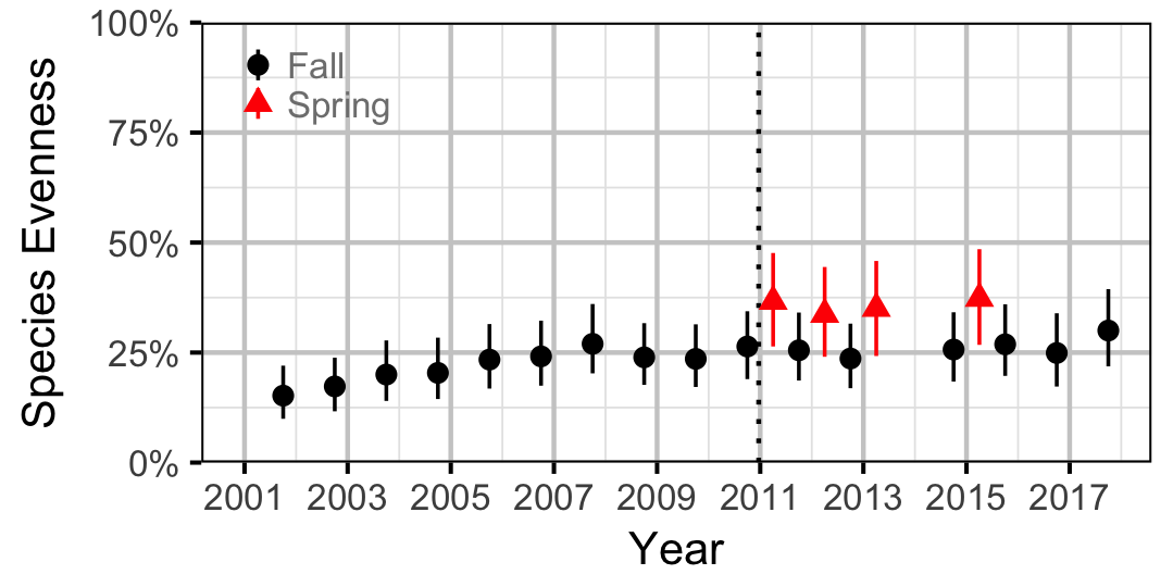
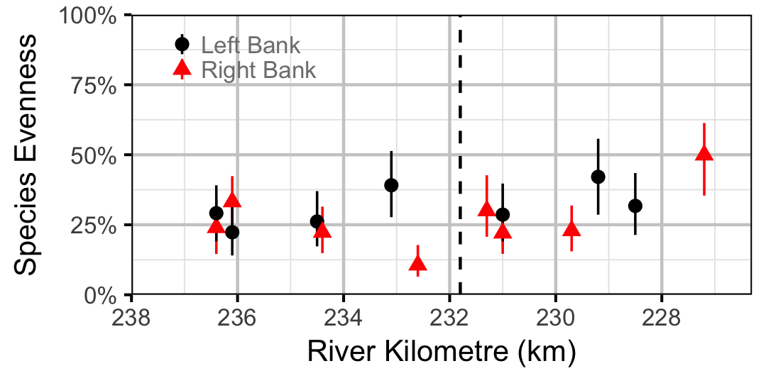
The site and year estimates of the lineal bank count densities from the count model for Rainbow Trout, Suckers, Burbot and Northern Pikeminnow were combined with the equivalent count estimates for Juvenile and Adult Bull Trout and Adult Mountain Whitefish from the abundance model to calculate the shannon index of evenness \((E)\). The index was calculated using the following formula where \(S\) is the number of species and \(p_i\) is the proportion of the total count belonging to the ith species.
\[ E = \frac{-\sum p_i \log(p_i)}{\log(S)}\]
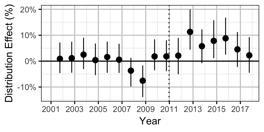
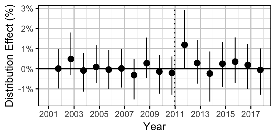
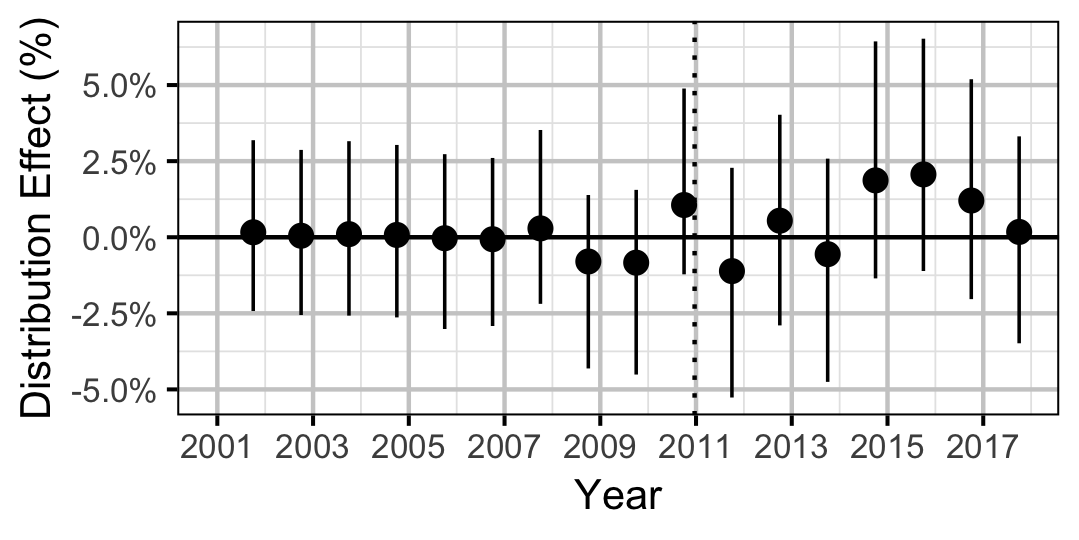
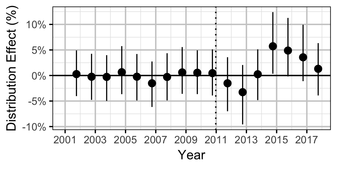
Distribution
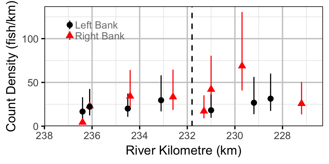
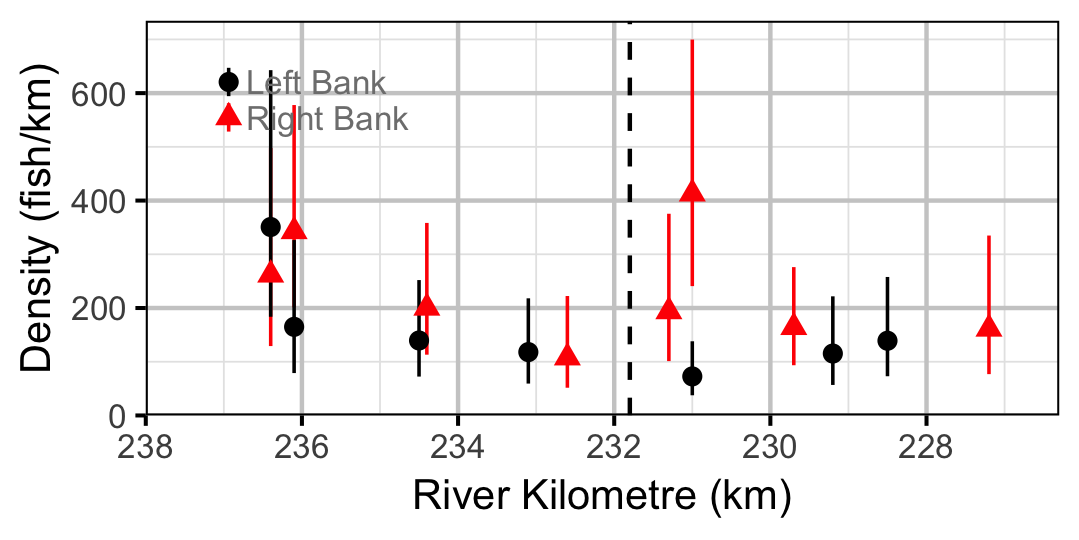
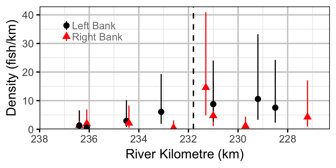
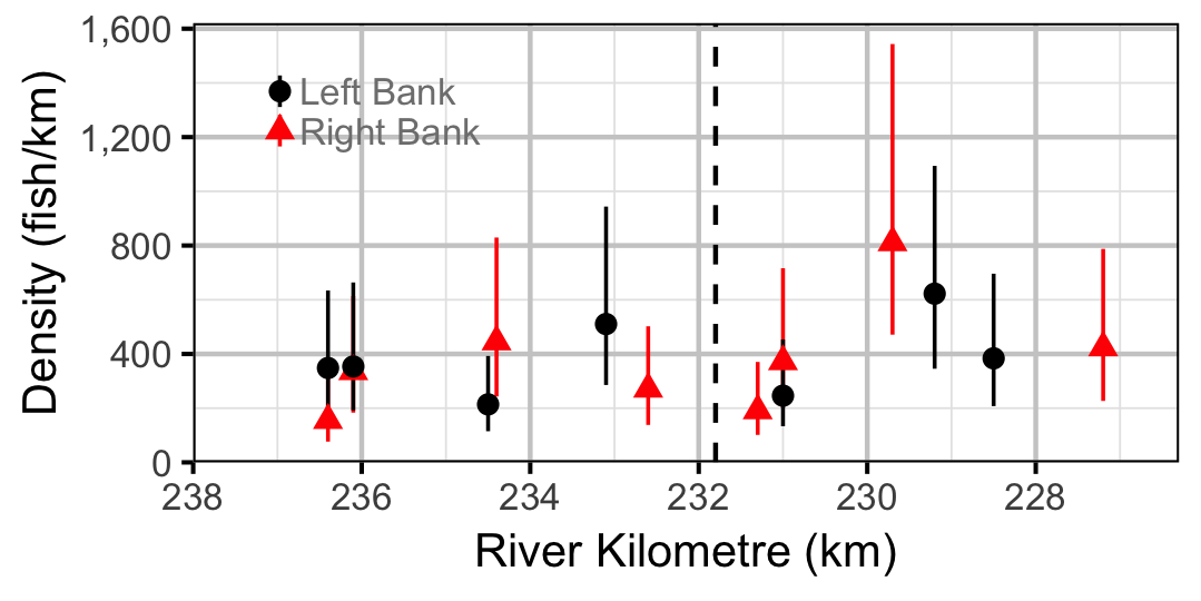
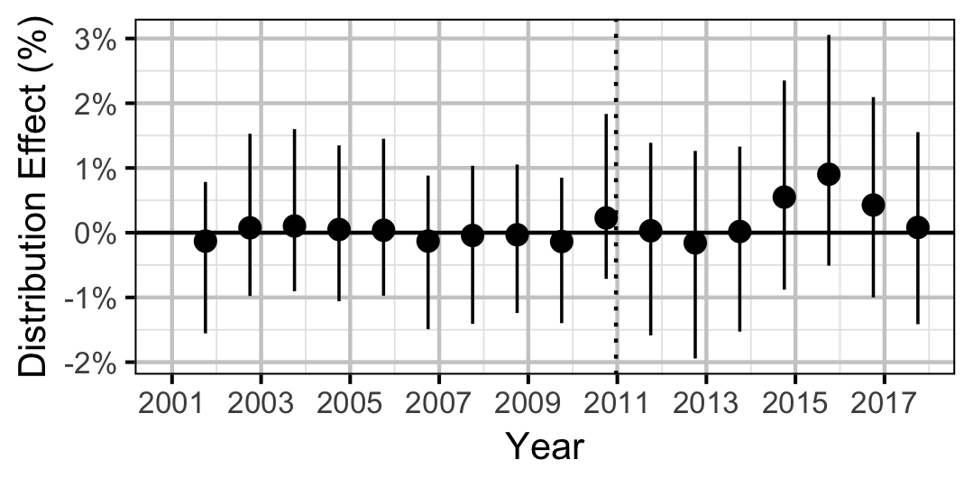
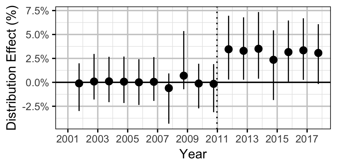
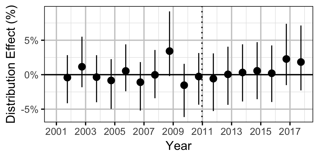
The site within year random effects from the count and abundance models were analysed using a linear mixed model to estimate the distribution.
Key assumptions of the linear mixed model include:
- The effect varies by river kilometer.
- The effect of river kilometer varies by discharge regime.
- The effect of river kilometer varies randomly by year.
- The effect is normally distributed.
The effects are the predicted site within year random effects after accounting for all other predictors including the site and year random effects. As such an increase in the distribution represents an increase in the relative density of fish closer to Mica Dam. A positive distribution does not however necessarily indicate that the density of fish is higher closer to Mica Dam.
Capture Effect
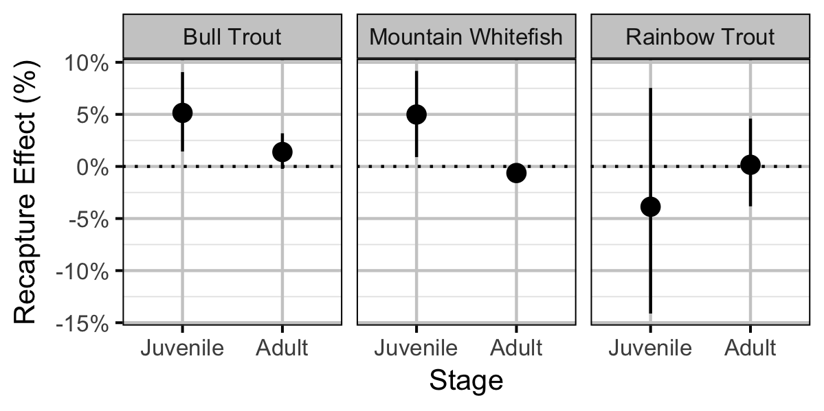
The effect of capture in a previous year was estimated via an analysis of mass-length relations (He et al. 2008).
Key assumptions of the capture effect model include:
- \(\alpha\) can vary with recapture and randomly with year.
- \(\beta\) can vary with recapture and randomly with year.
- The residual variation in weight is log-normally distributed.
Fry were excluded from the capture effect analysis.
Model Templates
Growth
model {

  bKIntercept ~ dnorm (0, 5^-2)

  bKRegime[1] <- 0
  for(i in 2:nRegime) {
    bKRegime[i] ~ dnorm(0, 5^-2)
  }

  sKAnnual ~ dunif(0, 5)
  for (i in 1:nAnnual) {
    bKAnnual[i] ~ dnorm(0, sKAnnual^-2)
    log(bK[i]) <- bKIntercept + bKRegime[step(i - Threshold) + 1] + bKAnnual[i]
  }

  bLinf ~ dunif(100,1000)
  sGrowth ~ dunif(0, 100)
  for (i in 1:length(Growth)) {

    eGrowth[i] <- (bLinf - LengthAtRelease[i]) * (1 - exp(-sum(bK[Annual[i]:(Annual[i] + Years[i] - 1)])))

    Growth[i] ~ dnorm(eGrowth[i], sGrowth^-2)
  }
  tGrowth <- bKRegime[2]
..
Template 1. The model description.
Condition
model {

  bWeightIntercept ~ dnorm(5, 5^-2)
  bWeightSlope ~ dnorm(3, 5^-2)

  bWeightRegimeIntercept[1] <- 0
  bWeightRegimeSlope[1] <- 0

  for(i in 2:nRegime) {
    bWeightRegimeIntercept[i] ~ dnorm(0, 5^-2)
    bWeightRegimeSlope[i] ~ dnorm(0, 5^-2)
  }

  bWeightSeasonIntercept[1] <- 0
  bWeightSeasonSlope[1] <- 0
  for(i in 2:nSeason) {
    bWeightSeasonIntercept[i] ~ dnorm(0, 5^-2)
    bWeightSeasonSlope[i] ~ dnorm(0, 5^-2)
  }

  sWeightYearIntercept ~ dunif(0, 1)
  sWeightYearSlope ~ dunif(0, 1)
  for(yr in 1:nYear) {
    bWeightYearIntercept[yr] ~ dnorm(0, sWeightYearIntercept^-2)
    bWeightYearSlope[yr] ~ dnorm(0, sWeightYearSlope^-2)
  }

  sWeight ~ dunif(0, 1)
  for(i in 1:length(Year)) {

    eWeightIntercept[i] <- bWeightIntercept + bWeightRegimeIntercept[Regime[i]] + bWeightSeasonIntercept[Season[i]] + bWeightYearIntercept[Year[i]]

    eWeightSlope[i] <- bWeightSlope + bWeightRegimeSlope[Regime[i]] + bWeightSeasonSlope[Season[i]] + bWeightYearSlope[Year[i]]

    log(eWeight[i]) <- eWeightIntercept[i] + eWeightSlope[i] * LogLength[i]
    Weight[i] ~ dlnorm(log(eWeight[i]) , sWeight^-2)
  }
  tCondition1 <- bWeightRegimeIntercept[2]
  tCondition2 <- bWeightRegimeSlope[2]
..
Template 2. The model description.
Occupancy
model {

  bRate ~ dnorm(0, 5^-2)

  sRateYear ~ dunif(0, 5)
  for(i in 1:nYear) {
    bRateYear[i] ~ dnorm(0, sRateYear^-2)
  }

  bRateRev5 ~ dnorm(0, 5^-2)

  bOccupancyYear[1] ~ dnorm(0, 5^-2)
  for (i in 2:nYear) {
    eRateYear[i-1] <- bRate + bRateYear[i-1] + bRateRev5 * YearRev5[i-1]
    bOccupancyYear[i] <- bOccupancyYear[i-1] + eRateYear[i-1]
  }

  bOccupancySpring ~ dnorm(0, 5^-2)

  sOccupancySite ~ dunif(0, 5)
  sOccupancySiteYear ~ dunif(0, 5)
  for (i in 1:nSite) {
    bOccupancySite[i] ~ dnorm(0, sOccupancySite^-2)
    for (j in 1:nYear) {
      bOccupancySiteYear[i,j] ~ dnorm(0, sOccupancySiteYear^-2)
    }
  }

  for (i in 1:length(Observed)) {
    logit(eObserved[i]) <- bOccupancyYear[Year[i]] + bOccupancySpring * Spring[i] + bOccupancySite[Site[i]] + bOccupancySiteYear[Site[i], Year[i]]
    Observed[i] ~ dbern(eObserved[i])
  }
..
Template 3. The model description.
Count
model {
  bDensity ~ dnorm(0, 5^-2)

  bRate ~ dnorm(0, 5^-2)
  bRateRev5 ~ dnorm(0, 5^-2)

  bTrendYear[1] <- bDensity
  for(i in 2:nYear) {
    bTrendYear[i] <- bTrendYear[i-1] + bRate + bRateRev5 * YearRev5[i-1]
  }

  bDensitySeason[1] <- 0
  for (i in 2:nSeason) {
    bDensitySeason[i] ~ dnorm(0, 5^-2)
  }

  sDensityYear ~ dunif(0, 5)
  for (i in 1:nYear) {
    bDensityYear[i] ~ dnorm(0, sDensityYear^-2)
  }

  sDensitySite ~ dunif(0, 5)
  sDensitySiteYear ~ dunif(0, 2)
  for (i in 1:nSite) {
    bDensitySite[i] ~ dnorm(0, sDensitySite^-2)
    for (j in 1:nYear) {
      bDensitySiteYear[i, j] ~ dnorm(0, sDensitySiteYear^-2)
    }
  }

  sDispersion ~ dunif(0, 5)
  for (i in 1:length(Year)) {

    log(eDensity[i]) <- bTrendYear[Year[i]] + bDensitySeason[Season[i]] + bDensityYear[Year[i]] + bDensitySite[Site[i]] + bDensitySiteYear[Site[i],Year[i]]

    eCount[i] <- eDensity[i] * SiteLength[i] * ProportionSampled[i]
    eDispersion[i] ~ dgamma(1 / sDispersion^2, 1 / sDispersion^2)
    Count[i] ~ dpois(eCount[i] * eDispersion[i])
  }
  tCount <- bRateRev5
..
Template 4. The model description.
Movement
model {
  bMoved ~ dnorm(0, 5^-2)
  bLength ~ dnorm(0, 5^-2)

  bMovedSpring ~ dnorm(0, 5^-5)
  bLengthSpring ~ dnorm(0, 5^-5)

  for (i in 1:length(Moved)) {
    logit(eMoved[i]) <- bMoved + bMovedSpring * Spring[i] + (bLength + bLengthSpring * Spring[i]) * Length[i]
    Moved[i] ~ dbern(eMoved[i])
  }
..
Template 5.
Abundance
model {
  bDensity ~ dnorm(0, 5^-2)

  bRate ~ dnorm(0, 5^-2)
  bRateRev5 ~ dnorm(0, 5^-2)

  bTrendYear[1] <- bDensity
  for(i in 2:nYear) {
    bTrendYear[i] <- bTrendYear[i-1] + bRate + bRateRev5 * YearRev5[i-1]
  }

  bDensitySeason[1] <- 0
  for (i in 2:nSeason) {
    bDensitySeason[i] ~ dnorm(0, 5^-2)
  }

  sDensityYear ~ dunif(0, 5)
  for (i in 1:nYear) {
    bDensityYear[i] ~ dnorm(0, sDensityYear^-2)
  }

  sDensitySite ~ dunif(0, 5)
  sDensitySiteYear ~ dunif(0, 2)
  for (i in 1:nSite) {
    bDensitySite[i] ~ dnorm(0, sDensitySite^-2)
    for (j in 1:nYear) {
      bDensitySiteYear[i, j] ~ dnorm(0, sDensitySiteYear^-2)
    }
  }

  bEfficiency ~ dnorm(0, 5^-2)

  bEfficiencySeason[1] <- 0
  for(i in 2:nSeason) {
    bEfficiencySeason[i] ~ dnorm(0, 5^-2)
  }

  sEfficiencySessionSeasonYear ~ dunif(0, 5)
  for (i in 1:nSession) {
    for (j in 1:nSeason) {
      for (k in 1:nYear) {
        bEfficiencySessionSeasonYear[i, j, k] ~ dnorm(0, sEfficiencySessionSeasonYear^-2)
      }
    }
  }

  bMultiplier <- 0
  sDispersion ~ dnorm(0, 2^-2)
  bMultiplierType[1] <- 0
  sDispersionType[1] <- 0
  for (i in 2:nType) {
    bMultiplierType[i] ~ dnorm(0, 2^-2)
    sDispersionType[i] ~ dnorm(0, 2^-2)
  }

  for(i in 1:length(EffIndex)) {

    logit(eEff[i]) <- bEfficiency + bEfficiencySeason[Season[EffIndex[i]]] + bEfficiencySessionSeasonYear[Session[EffIndex[i]],Season[EffIndex[i]],Year[EffIndex[i]]]

    Marked[EffIndex[i]] ~ dbin(eEff[i], Tagged[EffIndex[i]])
  }

  for (i in 1:length(Year)) {

    logit(eEfficiency[i]) <- bEfficiency + bEfficiencySeason[Season[i]] + bEfficiencySessionSeasonYear[Session[i], Season[i], Year[i]]

    log(eDensity[i]) <- bTrendYear[Year[i]] + bDensitySeason[Season[i]] + bDensityYear[Year[i]] + bDensitySite[Site[i]] + bDensitySiteYear[Site[i],Year[i]]

    log(eMultiplier[i]) <- bMultiplier + bMultiplierType[Type[i]]

    eCatch[i] <- eDensity[i] * SiteLength[i] * ProportionSampled[i] * eEfficiency[i] * eMultiplier[i]

    log(esDispersion[i]) <- sDispersion + sDispersionType[Type[i]]

    eDispersion[i] ~ dgamma(esDispersion[i]^-2 + 0.1, esDispersion[i]^-2 + 0.1)

    Catch[i] ~ dpois(eCatch[i] * eDispersion[i])
  }
  tAbundance <- bRateRev5
..
Template 6. The model description.
Distribution
model {
  bEffect ~ dnorm(0, 1^-2)

  bRkm ~ dnorm(0, 1^-2)
  bRkmRev5 ~ dnorm(0, 1^-2)

  sRkmYear ~ dunif(0, 1)
  for(i in 1:nYear) {
    bRkmYear[i] ~ dnorm(0, sRkmYear^-2)
  }
  sEffect ~ dunif(0, 1)
  for(i in 1:length(Effect)) {
    eEffect[i] <- bEffect + (bRkm + bRkmRev5 * Rev5[i] + bRkmYear[Year[i]]) * Rkm[i]
    Effect[i] ~ dnorm(eEffect[i], sEffect^-2)
  }
tDistribution <- bRkmRev5
Template 7. The model description.
Capture Effect
model {

  bWeightIntercept ~ dnorm(5, 5^-2)
  bWeightSlope ~ dnorm(3, 5^-2)

  bWeightRecaptureIntercept ~ dnorm(0, 5^-2)
  bWeightRecaptureSlope ~ dnorm(0, 5^-2)

  sWeightYearIntercept ~ dunif(0, 1)
  sWeightYearSlope ~ dunif(0, 1)
  for(yr in 1:nYear) {
    bWeightYearIntercept[yr] ~ dnorm(0, sWeightYearIntercept^-2)
    bWeightYearSlope[yr] ~ dnorm(0, sWeightYearSlope^-2)
  }

  sWeight ~ dunif(0, 1)
  for(i in 1:length(Year)) {

    eWeightIntercept[i] <- bWeightIntercept + bWeightRecaptureIntercept * Recapture[i] + bWeightYearIntercept[Year[i]]

    eWeightSlope[i] <- bWeightSlope + bWeightRecaptureSlope * Recapture[i] + bWeightYearSlope[Year[i]]

    log(eWeight[i]) <- eWeightIntercept[i] + eWeightSlope[i] * LogLength[i]
    Weight[i] ~ dlnorm(log(eWeight[i]) , sWeight^-2)
  }
..
Template 8. The model description.
Results
Tables
Growth
Table 2. Parameter descriptions.
| Parameter | Description |
|---|---|
Annual[i] |
Year |
bK[i] |
Expected growth coefficient in the ith Annual |
bKAnnual[i] |
Effect of ith Annual on bKIntercept |
bKIntercept |
Intercept for log(bK) |
bKRegime[i] |
Effect of ith Regime on bKIntercept |
bLinf |
Mean maximum length |
eGrowth[i] |
Expected Growth of the ith fish |
Growth[i] |
Change in length of the ith fish between release
and recapture (mm) |
LengthAtRelease[i] |
Length of the ith fish when released (mm) |
sGrowth |
SD of residual variation about eGrowth |
sKAnnual |
SD of bKAnnual |
Threshold |
Last Annual of the first regime |
Years[i] |
Number of years between release and recapture for the
ith fish |
Bull Trout
Table 3. Model coefficients.
| term | estimate | sd | zscore | lower | upper | pvalue |
|---|---|---|---|---|---|---|
| bKIntercept | -1.7956959 | 0.1284305 | -13.9794886 | -2.0540450 | -1.5396733 | 0.0007 |
| bKRegime[2] | -0.0912346 | 0.1567313 | -0.5988029 | -0.4190079 | 0.2115069 | 0.5213 |
| bLinf | 857.9665612 | 27.7940935 | 30.9575116 | 812.2310329 | 921.8432641 | 0.0007 |
| sGrowth | 31.4871398 | 1.3689584 | 23.0327024 | 29.0637196 | 34.2841835 | 0.0007 |
| sKAnnual | 0.2723559 | 0.0814077 | 3.4909084 | 0.1612945 | 0.4917336 | 0.0007 |
| tGrowth | -0.0912346 | 0.1567313 | -0.5988029 | -0.4190079 | 0.2115069 | 0.5213 |
Table 4. Model summary.
| n | K | nchains | niters | nthin | ess | rhat | converged |
|---|---|---|---|---|---|---|---|
| 281 | 6 | 3 | 500 | 20 | 396 | 1.008 | TRUE |
Mountain Whitefish
Table 5. Model coefficients.
| term | estimate | sd | zscore | lower | upper | pvalue |
|---|---|---|---|---|---|---|
| bKIntercept | -1.6162822 | 0.1443185 | -11.1885157 | -1.8994488 | -1.3339485 | 7e-04 |
| bKRegime[2] | -0.0450868 | 0.2090726 | -0.2378948 | -0.4734291 | 0.3629789 | 8e-01 |
| bLinf | 281.0074443 | 2.4198200 | 116.1727774 | 276.7228666 | 286.3675546 | 7e-04 |
| sGrowth | 9.4054613 | 0.2196507 | 42.8348303 | 8.9891443 | 9.8458449 | 7e-04 |
| sKAnnual | 0.3205001 | 0.1061132 | 3.1836481 | 0.1857553 | 0.6071873 | 7e-04 |
| tGrowth | -0.0450868 | 0.2090726 | -0.2378948 | -0.4734291 | 0.3629789 | 8e-01 |
Table 6. Model summary.
| n | K | nchains | niters | nthin | ess | rhat | converged |
|---|---|---|---|---|---|---|---|
| 935 | 6 | 3 | 500 | 20 | 297 | 1.016 | TRUE |
Condition
Table 7. Parameter descriptions.
| Parameter | Description |
|---|---|
bWeightIntercept |
Intercept for eWeightIntercept |
bWeightRegimeIntercept[i] |
Effect of ith Regime on bWeightIntercept |
bWeightRegimeSlope[i] |
Effect of ith Regime on bWeightSlope |
bWeightSeasonIntercept[i] |
Effect of ith Season on bWeightIntercept |
bWeightSeasonSlope[i] |
Effect of ith Season on bWeightSlope |
bWeightSlope |
Intercept for eWeightSlope |
bWeightYearIntercept[i] |
Effect of ith Year on bWeightIntercept |
bWeightYearSlope[i] |
Random effect of ith Year on bWeightSlope |
eWeight[i] |
Expected Weight of the ith fish |
eWeightIntercept[i] |
Intercept for log(eWeight[i]) |
eWeightSlope[i] |
Effect of LogLength on eWeightIntercept |
LogLength[i] |
The centered log(Length) of the ith fish |
sWeight |
SD of residual variation about eWeight |
sWeightYearIntercept |
SD of bWeightYearIntercept |
sWeightYearSlope |
SD of bWeightYearSlope |
Weight[i] |
The Weight of the ith fish |
Bull Trout
Table 8. Model coefficients.
| term | estimate | sd | zscore | lower | upper | pvalue |
|---|---|---|---|---|---|---|
| bWeightIntercept | 6.8243606 | 0.0253906 | 268.7847230 | 6.7719023 | 6.8767147 | 0.0007 |
| bWeightRegimeIntercept[2] | -0.0768944 | 0.0381404 | -2.0031837 | -0.1536060 | 0.0005419 | 0.0533 |
| bWeightRegimeSlope[2] | 0.0428429 | 0.0539794 | 0.7708220 | -0.0580331 | 0.1502438 | 0.4173 |
| bWeightSeasonIntercept[2] | 0.0008678 | 0.0092726 | 0.1092891 | -0.0172720 | 0.0188264 | 0.9253 |
| bWeightSeasonSlope[2] | 0.0103707 | 0.0234042 | 0.4220702 | -0.0392083 | 0.0546331 | 0.6707 |
| bWeightSlope | 3.1662076 | 0.0361134 | 87.6425723 | 3.0926189 | 3.2310180 | 0.0007 |
| sWeight | 0.1390229 | 0.0017840 | 77.9473838 | 0.1355927 | 0.1426388 | 0.0007 |
| sWeightYearIntercept | 0.0722051 | 0.0165045 | 4.5222876 | 0.0502368 | 0.1137593 | 0.0007 |
| sWeightYearSlope | 0.0946811 | 0.0239326 | 4.0853900 | 0.0610342 | 0.1520444 | 0.0007 |
| tCondition1 | -0.0768944 | 0.0381404 | -2.0031837 | -0.1536060 | 0.0005419 | 0.0533 |
| tCondition2 | 0.0428429 | 0.0539794 | 0.7708220 | -0.0580331 | 0.1502438 | 0.4173 |
Table 9. Model summary.
| n | K | nchains | niters | nthin | ess | rhat | converged |
|---|---|---|---|---|---|---|---|
| 3258 | 11 | 3 | 500 | 200 | 754 | 1.003 | TRUE |
Mountain Whitefish
Table 10. Model coefficients.
| term | estimate | sd | zscore | lower | upper | pvalue |
|---|---|---|---|---|---|---|
| bWeightIntercept | 4.7862432 | 0.0148585 | 322.1398836 | 4.7574469 | 4.8162260 | 0.0007 |
| bWeightRegimeIntercept[2] | -0.0218116 | 0.0211631 | -1.0238196 | -0.0651567 | 0.0203540 | 0.2947 |
| bWeightRegimeSlope[2] | -0.0201777 | 0.0254613 | -0.7960493 | -0.0703478 | 0.0332107 | 0.4200 |
| bWeightSeasonIntercept[2] | -0.0435541 | 0.0039948 | -10.9416851 | -0.0519632 | -0.0360428 | 0.0007 |
| bWeightSeasonSlope[2] | -0.1017893 | 0.0178866 | -5.6753994 | -0.1363834 | -0.0660136 | 0.0007 |
| bWeightSlope | 3.2083898 | 0.0172953 | 185.4762398 | 3.1738205 | 3.2409857 | 0.0007 |
| sWeight | 0.1008014 | 0.0007951 | 126.7651238 | 0.0993111 | 0.1024102 | 0.0007 |
| sWeightYearIntercept | 0.0406962 | 0.0089241 | 4.7253528 | 0.0286757 | 0.0627911 | 0.0007 |
| sWeightYearSlope | 0.0392578 | 0.0122856 | 3.3364323 | 0.0215437 | 0.0685571 | 0.0007 |
| tCondition1 | -0.0218116 | 0.0211631 | -1.0238196 | -0.0651567 | 0.0203540 | 0.2947 |
| tCondition2 | -0.0201777 | 0.0254613 | -0.7960493 | -0.0703478 | 0.0332107 | 0.4200 |
Table 11. Model summary.
| n | K | nchains | niters | nthin | ess | rhat | converged |
|---|---|---|---|---|---|---|---|
| 7785 | 11 | 3 | 500 | 200 | 513 | 1.007 | TRUE |
Rainbow Trout
Table 12. Model coefficients.
| term | estimate | sd | zscore | lower | upper | pvalue |
|---|---|---|---|---|---|---|
| bWeightIntercept | 4.6820357 | 0.0170798 | 274.1729503 | 4.6505567 | 4.7174297 | 0.0007 |
| bWeightRegimeIntercept[2] | 0.0040558 | 0.0253178 | 0.1387943 | -0.0507592 | 0.0507072 | 0.8613 |
| bWeightRegimeSlope[2] | -0.0479584 | 0.0552192 | -0.8786936 | -0.1607130 | 0.0541165 | 0.3693 |
| bWeightSeasonIntercept[2] | -0.0796013 | 0.0155338 | -5.1305247 | -0.1086392 | -0.0504453 | 0.0007 |
| bWeightSeasonSlope[2] | 0.0190345 | 0.0410411 | 0.4682897 | -0.0626553 | 0.0988973 | 0.6333 |
| bWeightSlope | 3.0874338 | 0.0371693 | 83.0972535 | 3.0179776 | 3.1649307 | 0.0007 |
| sWeight | 0.1151905 | 0.0034649 | 33.2655912 | 0.1083669 | 0.1221184 | 0.0007 |
| sWeightYearIntercept | 0.0344663 | 0.0134846 | 2.6205188 | 0.0120005 | 0.0645733 | 0.0007 |
| sWeightYearSlope | 0.0756046 | 0.0253223 | 3.1043012 | 0.0362450 | 0.1362144 | 0.0007 |
| tCondition1 | 0.0040558 | 0.0253178 | 0.1387943 | -0.0507592 | 0.0507072 | 0.8613 |
| tCondition2 | -0.0479584 | 0.0552192 | -0.8786936 | -0.1607130 | 0.0541165 | 0.3693 |
Table 13. Model summary.
| n | K | nchains | niters | nthin | ess | rhat | converged |
|---|---|---|---|---|---|---|---|
| 589 | 11 | 3 | 500 | 200 | 1304 | 1.004 | TRUE |
Largescale Sucker
Table 14. Model coefficients.
| term | estimate | sd | zscore | lower | upper | pvalue |
|---|---|---|---|---|---|---|
| bWeightIntercept | 6.8162164 | 0.0288220 | 236.505860 | 6.7585239 | 6.8728955 | 7e-04 |
| bWeightSeasonIntercept[2] | 0.0216586 | 0.0053503 | 4.040487 | 0.0112316 | 0.0319146 | 7e-04 |
| bWeightSeasonSlope[2] | 0.1666632 | 0.0455712 | 3.646674 | 0.0743200 | 0.2572852 | 7e-04 |
| bWeightSlope | 2.8822666 | 0.0927258 | 31.084418 | 2.7014079 | 3.0613701 | 7e-04 |
| sWeight | 0.0840283 | 0.0012262 | 68.538023 | 0.0817101 | 0.0865267 | 7e-04 |
| sWeightYearIntercept | 0.0683926 | 0.0269849 | 2.765798 | 0.0414743 | 0.1472769 | 7e-04 |
| sWeightYearSlope | 0.2267932 | 0.0939117 | 2.644467 | 0.1311874 | 0.4870871 | 7e-04 |
Table 15. Model summary.
| n | K | nchains | niters | nthin | ess | rhat | converged |
|---|---|---|---|---|---|---|---|
| 2426 | 7 | 3 | 500 | 200 | 261 | 1.023 | TRUE |
Occupancy
Table 16. Parameter descriptions.
| Parameter | Description |
|---|---|
bOccupancySite[i] |
Effect of ith site on bOccupancyYear |
bOccupancySiteYear[i,j] |
Effect of ith site in jth year on bOccupancyYear |
bOccupancySpring |
Effect of spring on bOccupancyYear |
bOccupancyYear[i] |
Expected Occupancy in ith year |
bRate |
Intercept of eRateYear |
bRateRev5[i] |
Effect of Revelstoke 5 regime on bRate |
bRateYear[i] |
Effect of ith year on biRate |
eObserved[i] |
Probability of observing a species on ith site visit |
eRateYear[i] |
Change in bOccupancyYear between year i-1 and year i |
Observed[i] |
Whether the species was observed on ith site visit |
sOccupancySite |
SD of bOccupancySite |
sOccupancySiteYear |
SD of bOccupancySiteYear |
sRateYear |
SD of bRateYear |
Rainbow Trout
Table 17. Model coefficients.
| term | estimate | sd | zscore | lower | upper | pvalue |
|---|---|---|---|---|---|---|
| bOccupancySpring | -0.0411117 | 0.2851908 | -0.1445481 | -0.6069750 | 0.5131999 | 0.8933 |
| bRate | 0.2379924 | 0.3928192 | 0.6185457 | -0.5593954 | 1.0582669 | 0.4787 |
| bRateRev5 | -0.2563198 | 0.6485588 | -0.3825753 | -1.5372282 | 1.0985291 | 0.6293 |
| sOccupancySite | 2.2264129 | 0.5430082 | 4.2772283 | 1.4887948 | 3.6018555 | 0.0007 |
| sOccupancySiteYear | 0.6653187 | 0.1947305 | 3.3943500 | 0.2568279 | 1.0403358 | 0.0007 |
| sRateYear | 1.1222808 | 0.3921133 | 3.0123116 | 0.6064728 | 2.1207664 | 0.0007 |
Table 18. Model summary.
| n | K | nchains | niters | nthin | ess | rhat | converged |
|---|---|---|---|---|---|---|---|
| 1014 | 6 | 3 | 500 | 1000 | 435 | 1.005 | TRUE |
Burbot
Table 19. Model coefficients.
| term | estimate | sd | zscore | lower | upper | pvalue |
|---|---|---|---|---|---|---|
| bOccupancySpring | -0.5057937 | 0.3223352 | -1.570036 | -1.1209661 | 0.1464580 | 0.1173 |
| bRate | 0.3841475 | 0.3898402 | 1.026790 | -0.3835111 | 1.2055886 | 0.2627 |
| bRateRev5 | -0.7194367 | 0.6396951 | -1.127059 | -1.9569717 | 0.5631416 | 0.2320 |
| sOccupancySite | 0.9911525 | 0.2835094 | 3.634356 | 0.5999947 | 1.6929255 | 0.0007 |
| sOccupancySiteYear | 0.4851008 | 0.2244312 | 2.146587 | 0.0592532 | 0.9056742 | 0.0007 |
| sRateYear | 1.1573749 | 0.3639998 | 3.306197 | 0.6403933 | 2.0551181 | 0.0007 |
Table 20. Model summary.
| n | K | nchains | niters | nthin | ess | rhat | converged |
|---|---|---|---|---|---|---|---|
| 1014 | 6 | 3 | 500 | 1000 | 512 | 1.007 | TRUE |
Lake Whitefish
Table 21. Model coefficients.
| term | estimate | sd | zscore | lower | upper | pvalue |
|---|---|---|---|---|---|---|
| bOccupancySpring | -4.8792868 | 0.7949583 | -6.2300809 | -6.6843511 | -3.5353613 | 0.0007 |
| bRate | 0.2280765 | 0.5909454 | 0.3487796 | -0.9741561 | 1.3314284 | 0.6947 |
| bRateRev5 | -0.4705963 | 0.9543082 | -0.4849325 | -2.3613754 | 1.5669143 | 0.5813 |
| sOccupancySite | 0.4622837 | 0.1803607 | 2.6677588 | 0.1831738 | 0.9018900 | 0.0007 |
| sOccupancySiteYear | 0.2073502 | 0.1679960 | 1.4007475 | 0.0069089 | 0.6153061 | 0.0007 |
| sRateYear | 1.7337401 | 0.4500629 | 3.9998384 | 1.1293434 | 2.8731815 | 0.0007 |
Table 22. Model summary.
| n | K | nchains | niters | nthin | ess | rhat | converged |
|---|---|---|---|---|---|---|---|
| 1014 | 6 | 3 | 500 | 1000 | 222 | 1.008 | TRUE |
Northern Pikeminnow
Table 23. Model coefficients.
| term | estimate | sd | zscore | lower | upper | pvalue |
|---|---|---|---|---|---|---|
| bOccupancySpring | -2.1728525 | 0.4525899 | -4.827522 | -3.1290960 | -1.3433385 | 0.0007 |
| bRate | 0.3630713 | 0.3090265 | 1.218756 | -0.1835884 | 1.0132314 | 0.1960 |
| bRateRev5 | -0.5877584 | 0.4778209 | -1.242252 | -1.5534644 | 0.3123419 | 0.1973 |
| sOccupancySite | 1.3978357 | 0.3928139 | 3.706250 | 0.8555126 | 2.3903382 | 0.0007 |
| sOccupancySiteYear | 0.7004825 | 0.2643190 | 2.594307 | 0.1236359 | 1.1938915 | 0.0007 |
| sRateYear | 0.7594259 | 0.3034616 | 2.640950 | 0.3173491 | 1.4880743 | 0.0007 |
Table 24. Model summary.
| n | K | nchains | niters | nthin | ess | rhat | converged |
|---|---|---|---|---|---|---|---|
| 1014 | 6 | 3 | 500 | 1000 | 786 | 1.007 | TRUE |
Redside Shiner
Table 25. Model coefficients.
| term | estimate | sd | zscore | lower | upper | pvalue |
|---|---|---|---|---|---|---|
| bOccupancySpring | -0.9326677 | 0.3716394 | -2.5384802 | -1.6948440 | -0.2119687 | 0.0120 |
| bRate | 0.3963091 | 0.4917673 | 0.8349994 | -0.5738027 | 1.4075349 | 0.3733 |
| bRateRev5 | -0.4400885 | 0.8081807 | -0.5668822 | -2.0794312 | 1.1450343 | 0.5467 |
| sOccupancySite | 2.1844716 | 0.5946516 | 3.8517367 | 1.4153988 | 3.6607364 | 0.0007 |
| sOccupancySiteYear | 0.3049922 | 0.2091674 | 1.5709232 | 0.0180595 | 0.7842232 | 0.0007 |
| sRateYear | 1.4353385 | 0.4748746 | 3.1669575 | 0.7826002 | 2.6408668 | 0.0007 |
Table 26. Model summary.
| n | K | nchains | niters | nthin | ess | rhat | converged |
|---|---|---|---|---|---|---|---|
| 1014 | 6 | 3 | 500 | 1000 | 336 | 1.006 | TRUE |
Sculpins
Table 27. Model coefficients.
| term | estimate | sd | zscore | lower | upper | pvalue |
|---|---|---|---|---|---|---|
| bOccupancySpring | -0.4595474 | 0.2749237 | -1.665046 | -1.0020872 | 0.0935364 | 0.0960 |
| bRate | 0.5311123 | 0.4401942 | 1.214043 | -0.3183993 | 1.4311108 | 0.2120 |
| bRateRev5 | -0.8558022 | 0.6876453 | -1.240467 | -2.2513058 | 0.4497523 | 0.2040 |
| sOccupancySite | 1.2980388 | 0.3129102 | 4.306438 | 0.8795545 | 2.1233750 | 0.0007 |
| sOccupancySiteYear | 0.3318056 | 0.1960727 | 1.733583 | 0.0172489 | 0.7342655 | 0.0007 |
| sRateYear | 1.2760344 | 0.3633538 | 3.657467 | 0.7833359 | 2.2107150 | 0.0007 |
Table 28. Model summary.
| n | K | nchains | niters | nthin | ess | rhat | converged |
|---|---|---|---|---|---|---|---|
| 1014 | 6 | 3 | 500 | 1000 | 268 | 1.03 | TRUE |
Count
Table 29. Parameter descriptions.
| Parameter | Description |
|---|---|
bDensity |
bTrendYear in the first year |
bDensitySeason |
Effect of season on bTrendYear |
bDensitySite[i] |
Effect of ith site on bTrendYear |
bDensitySiteYear[i,j] |
Effect of ith site in jth year on
bDensityTrend |
bDensityYear[i] |
Effect of ith year on bTrendYear |
bRate |
Exponential population growth rate |
bRateRev5 |
Effect of Rev5 on bRate |
bTrendYear[i] |
The intercept for the log(eDensity) in the ith
year |
Count[i] |
Count on ith site visit |
eCount[i] |
Expected count on ith site visit |
eDensity[i] |
Expected lineal count density on ith site visit |
eDispersion[i] |
Overdispersion on ith site visit |
ProportionSampled[i] |
Proportion of site sampled on ith site visit |
sDensitySite |
SD of bDensitySite |
sDensitySiteYear |
SD of bDensitySiteYear |
sDensityYear |
SD of bDensityYear |
sDispersion[i] |
SD of eDispersion |
SiteLength[i] |
Length of site on ith site visit |
YearRev5[i] |
Whether the rate of change between the ith and
i+1th year is effectd by Rev5 |
Rainbow Trout
Table 30. Model coefficients.
| term | estimate | sd | zscore | lower | upper | pvalue |
|---|---|---|---|---|---|---|
| bDensity | -2.8612928 | 0.6970114 | -4.0992721 | -4.2818787 | -1.4976945 | 0.0007 |
| bDensitySeason[2] | -0.1091911 | 0.1605998 | -0.6741163 | -0.4193663 | 0.2085626 | 0.4933 |
| bRate | 0.2592875 | 0.0718788 | 3.6459558 | 0.1219630 | 0.4066084 | 0.0007 |
| bRateRev5 | -0.4701834 | 0.1602989 | -2.9593910 | -0.7737993 | -0.1595690 | 0.0067 |
| sDensitySite | 1.7162579 | 0.4379115 | 4.1112994 | 1.1593217 | 2.9045018 | 0.0007 |
| sDensitySiteYear | 0.7686949 | 0.0884909 | 8.7347477 | 0.6082854 | 0.9558580 | 0.0007 |
| sDensityYear | 0.6199756 | 0.2007822 | 3.2310252 | 0.3469152 | 1.1138997 | 0.0007 |
| sDispersion | 0.8183775 | 0.0555904 | 14.7819962 | 0.7198484 | 0.9350104 | 0.0007 |
| tCount | -0.4701834 | 0.1602989 | -2.9593910 | -0.7737993 | -0.1595690 | 0.0067 |
Table 31. Model summary.
| n | K | nchains | niters | nthin | ess | rhat | converged |
|---|---|---|---|---|---|---|---|
| 1014 | 9 | 3 | 500 | 2000 | 1098 | 1.004 | TRUE |
Burbot
Table 32. Model coefficients.
| term | estimate | sd | zscore | lower | upper | pvalue |
|---|---|---|---|---|---|---|
| bDensity | -3.2034164 | 0.7287912 | -4.440413 | -4.7488911 | -1.9144469 | 0.0007 |
| bDensitySeason[2] | -0.7552142 | 0.2818057 | -2.681966 | -1.3239397 | -0.2138741 | 0.0080 |
| bRate | 0.2346567 | 0.1037963 | 2.294250 | 0.0433189 | 0.4662045 | 0.0213 |
| bRateRev5 | -0.7258272 | 0.2543536 | -2.875374 | -1.2534283 | -0.2235450 | 0.0027 |
| sDensitySite | 0.7945730 | 0.2324992 | 3.547255 | 0.4679400 | 1.3718340 | 0.0007 |
| sDensitySiteYear | 0.4101321 | 0.1919138 | 2.072994 | 0.0375071 | 0.7548380 | 0.0007 |
| sDensityYear | 0.9986961 | 0.3129010 | 3.290181 | 0.5483730 | 1.7289211 | 0.0007 |
| sDispersion | 1.1998372 | 0.1370626 | 8.780270 | 0.9424904 | 1.4752871 | 0.0007 |
| tCount | -0.7258272 | 0.2543536 | -2.875374 | -1.2534283 | -0.2235450 | 0.0027 |
Table 33. Model summary.
| n | K | nchains | niters | nthin | ess | rhat | converged |
|---|---|---|---|---|---|---|---|
| 1014 | 9 | 3 | 500 | 2000 | 1014 | 1.005 | TRUE |
Northern Pikeminnow
Table 34. Model coefficients.
| term | estimate | sd | zscore | lower | upper | pvalue |
|---|---|---|---|---|---|---|
| bDensity | -4.3557727 | 0.8407470 | -5.234004 | -6.1851440 | -2.8834448 | 7e-04 |
| bDensitySeason[2] | -2.3944693 | 0.4384267 | -5.516285 | -3.3346633 | -1.6149347 | 7e-04 |
| bRate | 0.3592536 | 0.1022956 | 3.581009 | 0.1916289 | 0.5831458 | 7e-04 |
| bRateRev5 | -0.6998474 | 0.2070067 | -3.445488 | -1.1535332 | -0.3364977 | 7e-04 |
| sDensitySite | 1.2799847 | 0.3761511 | 3.540258 | 0.7821973 | 2.2194469 | 7e-04 |
| sDensitySiteYear | 0.7345422 | 0.1922025 | 3.785029 | 0.3314408 | 1.0923605 | 7e-04 |
| sDensityYear | 0.6780051 | 0.2521644 | 2.834982 | 0.3235725 | 1.3141275 | 7e-04 |
| sDispersion | 1.3407643 | 0.1309785 | 10.242386 | 1.0931417 | 1.6039903 | 7e-04 |
| tCount | -0.6998474 | 0.2070067 | -3.445488 | -1.1535332 | -0.3364977 | 7e-04 |
Table 35. Model summary.
| n | K | nchains | niters | nthin | ess | rhat | converged |
|---|---|---|---|---|---|---|---|
| 1014 | 9 | 3 | 500 | 2000 | 1168 | 1.005 | TRUE |
Suckers
Table 36. Model coefficients.
| term | estimate | sd | zscore | lower | upper | pvalue |
|---|---|---|---|---|---|---|
| bDensity | 1.9658082 | 0.2534481 | 7.751190 | 1.4894203 | 2.4691617 | 0.0007 |
| bDensityRev5 | 0.7222453 | 0.3159206 | 2.274950 | 0.1196108 | 1.3601837 | 0.0240 |
| bDensitySeason[2] | -0.3241030 | 0.1006812 | -3.248471 | -0.5247304 | -0.1289312 | 0.0007 |
| sDensitySite | 0.5236664 | 0.1315783 | 4.135944 | 0.3458364 | 0.8429951 | 0.0007 |
| sDensitySiteYear | 0.5071496 | 0.0472447 | 10.735497 | 0.4187704 | 0.6020424 | 0.0007 |
| sDensityYear | 0.5781484 | 0.1352985 | 4.428347 | 0.3953560 | 0.9251016 | 0.0007 |
| sDispersion | 0.7576635 | 0.0228915 | 33.138315 | 0.7139924 | 0.8059571 | 0.0007 |
| tCount | 0.7222453 | 0.3159206 | 2.274950 | 0.1196108 | 1.3601837 | 0.0240 |
Table 37. Model summary.
| n | K | nchains | niters | nthin | ess | rhat | converged |
|---|---|---|---|---|---|---|---|
| 1014 | 8 | 3 | 500 | 2000 | 894 | 1.005 | TRUE |
Movement
Table 38. Parameter descriptions.
| Parameter | Description |
|---|---|
bLength |
Effect of Length on bMoved |
bLengthSpring |
Effect of Spring on bLength |
bMoved |
Intercept for logit(eMoved) |
bMovedSpring |
Effect of Spring on bMoved |
eMoved[i] |
Probability of different site from previous encounter for
ith recaptured fish |
Length[i] |
Length of ith recaptured fish (mm) |
Moved[i] |
Indicates whether ith recaptured fish is recorded at a
different site from previous encounter |
Spring[i] |
Whether the ith recaptured is from the spring |
Bull Trout
Table 39. Model coefficients.
| term | estimate | sd | zscore | lower | upper | pvalue |
|---|---|---|---|---|---|---|
| bLength | 0.0050472 | 0.0016056 | 3.1326266 | 0.0018442 | 0.0082599 | 0.0013 |
| bLengthSpring | 0.0019111 | 0.0062901 | 0.3996867 | -0.0085459 | 0.0168717 | 0.7373 |
| bMoved | -2.0057737 | 0.7198206 | -2.7697381 | -3.4094842 | -0.5923852 | 0.0053 |
| bMovedSpring | 0.0193226 | 2.7084371 | -0.0445004 | -6.0079853 | 4.7805567 | 0.9960 |
Table 40. Model summary.
| n | K | nchains | niters | nthin | ess | rhat | converged |
|---|---|---|---|---|---|---|---|
| 144 | 4 | 3 | 500 | 100 | 1314 | 1.002 | TRUE |
Mountain Whitefish
Table 41. Model coefficients.
| term | estimate | sd | zscore | lower | upper | pvalue |
|---|---|---|---|---|---|---|
| bLength | -0.0012623 | 0.0028729 | -0.4149524 | -0.0067981 | 0.0042952 | 0.6827 |
| bLengthSpring | -0.0265964 | 0.0068067 | -3.9631561 | -0.0403634 | -0.0141731 | 0.0007 |
| bMoved | 0.2354738 | 0.7347255 | 0.2992118 | -1.1754436 | 1.6778067 | 0.7680 |
| bMovedSpring | 5.4685838 | 1.6255916 | 3.4274672 | 2.4814080 | 8.8208538 | 0.0007 |
Table 42. Model summary.
| n | K | nchains | niters | nthin | ess | rhat | converged |
|---|---|---|---|---|---|---|---|
| 459 | 4 | 3 | 500 | 100 | 555 | 1.002 | TRUE |
Rainbow Trout
Table 43. Model coefficients.
| term | estimate | sd | zscore | lower | upper | pvalue |
|---|---|---|---|---|---|---|
| bLength | 0.0108561 | 0.0060665 | 1.817775 | -0.0000668 | 0.0230225 | 0.0520 |
| bLengthSpring | 0.2187275 | 0.1219674 | 1.899689 | 0.0294910 | 0.5034065 | 0.0133 |
| bMoved | -3.2979571 | 1.6582649 | -2.013013 | -6.8102456 | -0.4088259 | 0.0240 |
| bMovedSpring | -66.6287828 | 36.3791852 | -1.944310 | -151.3493832 | -10.0658893 | 0.0120 |
Table 44. Model summary.
| n | K | nchains | niters | nthin | ess | rhat | converged |
|---|---|---|---|---|---|---|---|
| 25 | 4 | 3 | 500 | 100 | 448 | 1.004 | TRUE |
Largescale Sucker
Table 45. Model coefficients.
| term | estimate | sd | zscore | lower | upper | pvalue |
|---|---|---|---|---|---|---|
| bLength | -0.0098648 | 0.0057419 | -1.732708 | -0.0209798 | 0.0003701 | 0.0613 |
| bLengthSpring | -0.1755000 | 0.0805597 | -2.232773 | -0.3441619 | -0.0406039 | 0.0053 |
| bMoved | 4.1410501 | 2.4908500 | 1.656872 | -0.3073915 | 8.9910564 | 0.0773 |
| bMovedSpring | 77.2610292 | 35.4047315 | 2.231718 | 17.1950237 | 150.8352660 | 0.0067 |
Table 46. Model summary.
| n | K | nchains | niters | nthin | ess | rhat | converged |
|---|---|---|---|---|---|---|---|
| 72 | 4 | 3 | 500 | 200 | 162 | 1.018 | TRUE |
Abundance
Table 47. Parameter descriptions.
| Parameter | Description |
|---|---|
bDensity |
Intercept for log(eDensity) in the 1st year |
bDensitySeason[i] |
Effect of ith season on bTrendYear |
bDensitySite[i] |
Effect of ith site on bDensity |
bDensitySiteYear[i,j] |
Effect of ith site in jth year on
bDensity |
bDensityYear[i] |
Effect of ith year on bDensity |
bEfficiency |
Intercept for logit(eEfficiency) |
bEfficiencySeason[i] |
Effect of ith season on bEfficiency |
bEfficiencySessionSeasonYear[i, j, k] |
Effect of ith Session in jth Season
of kth Year on bEfficiency |
bRate |
Exponential annual population growth rate |
bRateRev5[i] |
Effect of Rev5 on bRate |
bTrendYear[i] |
Intercept for log(eDensity) in the ith
year |
Catch[i] |
Number of fish caught on ith site visit |
eAbundance[i] |
Predicted abundance on ith site visit |
eDensity[i] |
Predicted lineal density on ith site visit |
eEfficiency[i] |
Predicted efficiency during ith site visit |
Marked[i] |
Number of marked fish caught in ith river
visit |
sDensitySite |
SD of bDensitySite |
sDensitySiteYear |
SD of bDensitySiteYear |
sDensityYear |
SD of bDensityYear |
sEfficiencySessionSeasonYear |
SD of bEfficiencySessionSeasonYear |
Tagged[i] |
Number of fish tagged prior to ith river
visit |
Bull Trout
Juvenile
Table 48. Model coefficients.
| term | estimate | sd | zscore | lower | upper | pvalue |
|---|---|---|---|---|---|---|
| bDensity | 2.0317352 | 0.3790120 | 5.3455424 | 1.3033732 | 2.7645543 | 0.0007 |
| bDensitySeason[2] | 0.2440742 | 0.3530140 | 0.7338443 | -0.4119758 | 1.0001333 | 0.4760 |
| bEfficiency | -3.1353008 | 0.1432960 | -21.9225965 | -3.4353124 | -2.8794709 | 0.0007 |
| bEfficiencySeason[2] | -0.3537353 | 0.3604264 | -1.0139636 | -1.0918352 | 0.3142488 | 0.3093 |
| bMultiplierType[2] | 0.2722326 | 0.1713857 | 1.5890810 | -0.0464302 | 0.6271081 | 0.1053 |
| bRate | 0.1491630 | 0.0465825 | 3.2319406 | 0.0643235 | 0.2508200 | 0.0013 |
| bRateRev5 | -0.1868586 | 0.1138132 | -1.6729114 | -0.4362648 | 0.0249896 | 0.0760 |
| sDensitySite | 0.6001291 | 0.1445960 | 4.2988961 | 0.3989052 | 0.9574976 | 0.0007 |
| sDensitySiteYear | 0.2773329 | 0.0584176 | 4.7249048 | 0.1550644 | 0.3873249 | 0.0007 |
| sDensityYear | 0.4398299 | 0.1276335 | 3.5747469 | 0.2472924 | 0.7536640 | 0.0007 |
| sDispersion | -0.9601223 | 0.1475537 | -6.5768298 | -1.2822591 | -0.7199343 | 0.0007 |
| sDispersionType[2] | 0.5865248 | 0.2832811 | 2.0246163 | -0.0040704 | 1.0888026 | 0.0507 |
| sEfficiencySessionSeasonYear | 0.2361710 | 0.0521742 | 4.5320186 | 0.1365222 | 0.3407249 | 0.0007 |
| tAbundance | -0.1868586 | 0.1138132 | -1.6729114 | -0.4362648 | 0.0249896 | 0.0760 |
Table 49. Model summary.
| n | K | nchains | niters | nthin | ess | rhat | converged |
|---|---|---|---|---|---|---|---|
| 1104 | 14 | 3 | 500 | 2000 | 1132 | 1.005 | TRUE |
Adult
Table 50. Model coefficients.
| term | estimate | sd | zscore | lower | upper | pvalue |
|---|---|---|---|---|---|---|
| bDensity | 4.1205850 | 0.2637881 | 15.6250993 | 3.6079347 | 4.6517529 | 0.0007 |
| bDensitySeason[2] | -0.1943602 | 0.3581661 | -0.5225600 | -0.8562970 | 0.5597798 | 0.5560 |
| bEfficiency | -3.6315919 | 0.1165034 | -31.1930482 | -3.8700865 | -3.4163559 | 0.0007 |
| bEfficiencySeason[2] | -0.0857431 | 0.3557813 | -0.2745795 | -0.8368120 | 0.5837932 | 0.8013 |
| bMultiplierType[2] | 0.5222438 | 0.1493106 | 3.5334669 | 0.2390014 | 0.8266887 | 0.0007 |
| bRate | 0.0272884 | 0.0291399 | 0.9630816 | -0.0269118 | 0.0869345 | 0.2973 |
| bRateRev5 | -0.0332167 | 0.0693881 | -0.4786373 | -0.1633932 | 0.1056415 | 0.6053 |
| sDensitySite | 0.5451917 | 0.1340689 | 4.2043831 | 0.3547699 | 0.8838168 | 0.0007 |
| sDensitySiteYear | 0.4149849 | 0.0423970 | 9.7917041 | 0.3344406 | 0.5012764 | 0.0007 |
| sDensityYear | 0.2365239 | 0.0957466 | 2.4939250 | 0.0538772 | 0.4514469 | 0.0007 |
| sDispersion | -0.9190190 | 0.0925200 | -9.9944092 | -1.1148555 | -0.7559762 | 0.0007 |
| sDispersionType[2] | 0.4416597 | 0.1880097 | 2.3195082 | 0.0221530 | 0.7859473 | 0.0387 |
| sEfficiencySessionSeasonYear | 0.2178296 | 0.0428757 | 5.1497094 | 0.1426023 | 0.3132982 | 0.0007 |
| tAbundance | -0.0332167 | 0.0693881 | -0.4786373 | -0.1633932 | 0.1056415 | 0.6053 |
Table 51. Model summary.
| n | K | nchains | niters | nthin | ess | rhat | converged |
|---|---|---|---|---|---|---|---|
| 1104 | 14 | 3 | 500 | 2000 | 1174 | 1.005 | TRUE |
Mountain Whitefish
Juvenile
Table 52. Model coefficients.
| term | estimate | sd | zscore | lower | upper | pvalue |
|---|---|---|---|---|---|---|
| bDensity | 5.6170627 | 0.6690741 | 8.4116993 | 4.3434876 | 6.9734945 | 0.0007 |
| bDensitySeason[2] | 0.4646623 | 0.6886065 | 0.6547951 | -0.8827184 | 1.8198348 | 0.5093 |
| bEfficiency | -5.7262786 | 0.4371984 | -13.1478443 | -6.6739146 | -4.9536452 | 0.0007 |
| bEfficiencySeason[2] | 0.0488543 | 0.6901959 | 0.0807100 | -1.3351240 | 1.3632474 | 0.9413 |
| bMultiplierType[2] | 0.5330413 | 0.2124633 | 2.5013183 | 0.1138232 | 0.9556618 | 0.0133 |
| bRate | 0.0906223 | 0.1657261 | 0.5615328 | -0.2348045 | 0.4410380 | 0.5307 |
| bRateRev5 | -0.1350301 | 0.2425361 | -0.5677648 | -0.6479221 | 0.3228641 | 0.5307 |
| sDensitySite | 0.9003265 | 0.2198041 | 4.2653817 | 0.6121254 | 1.4376721 | 0.0007 |
| sDensitySiteYear | 0.5135963 | 0.0628418 | 8.1683567 | 0.3905679 | 0.6378851 | 0.0007 |
| sDensityYear | 0.5128644 | 0.2115669 | 2.6032595 | 0.2451370 | 1.0591084 | 0.0007 |
| sDispersion | -0.5576387 | 0.0882409 | -6.3517525 | -0.7379878 | -0.3937922 | 0.0007 |
| sDispersionType[2] | 0.5531513 | 0.1672067 | 3.3127635 | 0.2398062 | 0.8928915 | 0.0013 |
| sEfficiencySessionSeasonYear | 0.2920152 | 0.0633951 | 4.6358054 | 0.1679092 | 0.4275948 | 0.0007 |
| tAbundance | -0.1350301 | 0.2425361 | -0.5677648 | -0.6479221 | 0.3228641 | 0.5307 |
Table 53. Model summary.
| n | K | nchains | niters | nthin | ess | rhat | converged |
|---|---|---|---|---|---|---|---|
| 875 | 14 | 3 | 500 | 2000 | 498 | 1.005 | TRUE |
Adult
Table 54. Model coefficients.
| term | estimate | sd | zscore | lower | upper | pvalue |
|---|---|---|---|---|---|---|
| bDensity | 6.6878660 | 0.1980319 | 33.7641948 | 6.3013714 | 7.0956635 | 0.0007 |
| bDensitySeason[2] | -0.6542806 | 0.1223199 | -5.3626028 | -0.9068309 | -0.4196073 | 0.0007 |
| bEfficiency | -4.0065177 | 0.0662289 | -60.5198737 | -4.1382706 | -3.8784746 | 0.0007 |
| bEfficiencySeason[2] | 0.9042058 | 0.1217576 | 7.4409046 | 0.6770769 | 1.1561322 | 0.0007 |
| bMultiplierType[2] | 0.7479242 | 0.1463030 | 5.1066947 | 0.4445880 | 1.0248355 | 0.0007 |
| bRate | 0.0018701 | 0.0187605 | 0.1198861 | -0.0368802 | 0.0388578 | 0.9013 |
| bRateRev5 | -0.0270408 | 0.0446637 | -0.6070068 | -0.1143601 | 0.0595042 | 0.5253 |
| sDensitySite | 0.5486478 | 0.1285072 | 4.4492360 | 0.3718853 | 0.8654625 | 0.0007 |
| sDensitySiteYear | 0.3960126 | 0.0301615 | 13.1675431 | 0.3396973 | 0.4586579 | 0.0007 |
| sDensityYear | 0.0820778 | 0.0591381 | 1.4821590 | 0.0025397 | 0.2202992 | 0.0007 |
| sDispersion | -0.7957032 | 0.0373020 | -21.3570001 | -0.8702372 | -0.7233282 | 0.0007 |
| sDispersionType[2] | 0.4181438 | 0.1028141 | 4.0723840 | 0.2249781 | 0.6182324 | 0.0007 |
| sEfficiencySessionSeasonYear | 0.2444777 | 0.0301583 | 8.1768445 | 0.1913308 | 0.3095988 | 0.0007 |
| tAbundance | -0.0270408 | 0.0446637 | -0.6070068 | -0.1143601 | 0.0595042 | 0.5253 |
Table 55. Model summary.
| n | K | nchains | niters | nthin | ess | rhat | converged |
|---|---|---|---|---|---|---|---|
| 1104 | 14 | 3 | 500 | 2000 | 927 | 1.006 | TRUE |
Rainbow Trout
Adult
Table 56. Model coefficients.
| term | estimate | sd | zscore | lower | upper | pvalue |
|---|---|---|---|---|---|---|
| bDensity | 0.4137203 | 0.5939575 | 0.6771314 | -0.8204313 | 1.5553675 | 0.4747 |
| bDensitySeason[2] | 0.2489691 | 0.6649070 | 0.4421001 | -0.8825792 | 1.7504814 | 0.7053 |
| bEfficiency | -2.4743420 | 0.2592588 | -9.5758978 | -3.0354726 | -2.0359383 | 0.0007 |
| bEfficiencySeason[2] | -0.5358472 | 0.6659936 | -0.8717729 | -2.0607134 | 0.5551417 | 0.3760 |
| bMultiplierType[2] | 0.0452367 | 2.0116422 | 0.0226372 | -3.8948973 | 3.9903901 | 0.9840 |
| bRate | -0.0230432 | 0.1597252 | -0.1611414 | -0.3559728 | 0.2931614 | 0.8747 |
| bRateRev5 | 0.1443743 | 0.2352091 | 0.6007055 | -0.3529188 | 0.6400748 | 0.5187 |
| sDensitySite | 1.2130851 | 0.3312549 | 3.8168251 | 0.7689813 | 2.0414908 | 0.0007 |
| sDensitySiteYear | 0.5868438 | 0.1349415 | 4.3561290 | 0.3375407 | 0.8529505 | 0.0007 |
| sDensityYear | 0.4177111 | 0.2376546 | 1.8522135 | 0.0485949 | 0.9405130 | 0.0007 |
| sDispersion | -1.6241304 | 1.1805303 | -1.6332341 | -4.9241527 | -0.4965307 | 0.0007 |
| sDispersionType[2] | -0.1364874 | 2.0229551 | -0.0361438 | -3.9223618 | 3.8385929 | 0.9560 |
| sEfficiencySessionSeasonYear | 0.2860454 | 0.1373747 | 2.0540970 | 0.0246497 | 0.5506224 | 0.0007 |
| tAbundance | 0.1443743 | 0.2352091 | 0.6007055 | -0.3529188 | 0.6400748 | 0.5187 |
Table 57. Model summary.
| n | K | nchains | niters | nthin | ess | rhat | converged |
|---|---|---|---|---|---|---|---|
| 785 | 14 | 3 | 500 | 2000 | 387 | 1.005 | TRUE |
Largescale Sucker
Adult
Table 58. Model coefficients.
| term | estimate | sd | zscore | lower | upper | pvalue |
|---|---|---|---|---|---|---|
| bDensity | 5.1510705 | 0.2876970 | 17.8987169 | 4.5985206 | 5.7082043 | 0.0007 |
| bDensitySeason[2] | 0.0157497 | 0.5749163 | 0.0847352 | -0.9717747 | 1.2267107 | 0.9800 |
| bEfficiency | -3.4600753 | 0.1590708 | -21.7684830 | -3.7810554 | -3.1537326 | 0.0007 |
| bEfficiencySeason[2] | -1.1800022 | 0.5871715 | -2.0659784 | -2.4420089 | -0.1310982 | 0.0213 |
| bMultiplierType[2] | 0.6759784 | 0.2512915 | 2.7451933 | 0.2144580 | 1.1928307 | 0.0027 |
| sDensitySite | 0.5096088 | 0.1319270 | 4.0098108 | 0.3292363 | 0.8546882 | 0.0007 |
| sDensitySiteYear | 0.4372796 | 0.0557146 | 7.8583799 | 0.3304168 | 0.5502250 | 0.0007 |
| sDensityYear | 0.5301892 | 0.2636274 | 2.2378175 | 0.2627932 | 1.2250619 | 0.0007 |
| sDispersion | -0.7241668 | 0.0737539 | -9.8319012 | -0.8701852 | -0.5836334 | 0.0007 |
| sDispersionType[2] | 0.3779230 | 0.1477453 | 2.5376958 | 0.0950942 | 0.6695803 | 0.0120 |
| sEfficiencySessionSeasonYear | 0.5334568 | 0.0873531 | 6.2060991 | 0.3921578 | 0.7318386 | 0.0007 |
Table 59. Model summary.
| n | K | nchains | niters | nthin | ess | rhat | converged |
|---|---|---|---|---|---|---|---|
| 660 | 11 | 3 | 500 | 2000 | 1212 | 1.005 | TRUE |
Distribution
Table 60. Parameter descriptions.
| Parameter | Description |
|---|---|
bEffect |
Intercept for eEffect |
bRkm |
Effect of Rkm on bEffect |
bRkmRev5 |
Effect of Rev5 on bRkm |
bRkmYear[i] |
Effect of ith year on bRkm |
eEffect |
Expected Effect |
Effect |
Estimated site and year effect from the count or abundance model |
Rkm |
Standardised river kilometre |
sEffect |
SD of residual variation in Effect |
sRkmYear |
SD of bRkmYear |
Bull Trout
Juvenile
Table 61. Model coefficients.
| term | estimate | sd | zscore | lower | upper | pvalue |
|---|---|---|---|---|---|---|
| bEffect | 0.0012219 | 0.0072488 | 0.1886369 | -0.0121164 | 0.0156917 | 0.8560 |
| bRkm | -0.0009996 | 0.0040039 | -0.2652176 | -0.0088620 | 0.0069872 | 0.7867 |
| bRkmRev5 | 0.0026939 | 0.0060819 | 0.4406870 | -0.0098143 | 0.0150106 | 0.6467 |
| sEffect | 0.1169748 | 0.0051791 | 22.6095410 | 0.1075126 | 0.1275491 | 0.0007 |
| sRkmYear | 0.0059504 | 0.0037622 | 1.6693618 | 0.0002967 | 0.0146578 | 0.0007 |
| tDistribution | 0.0026939 | 0.0060819 | 0.4406870 | -0.0098143 | 0.0150106 | 0.6467 |
Table 62. Model summary.
| n | K | nchains | niters | nthin | ess | rhat | converged |
|---|---|---|---|---|---|---|---|
| 255 | 6 | 3 | 500 | 10 | 330 | 1.01 | TRUE |
Adult
Table 63. Model coefficients.
| term | estimate | sd | zscore | lower | upper | pvalue |
|---|---|---|---|---|---|---|
| bEffect | 0.0021188 | 0.0162774 | 0.1475748 | -0.0292853 | 0.0339879 | 0.8960 |
| bRkm | -0.0101684 | 0.0085917 | -1.1827391 | -0.0267713 | 0.0067268 | 0.2267 |
| bRkmRev5 | 0.0313800 | 0.0136076 | 2.2969018 | 0.0036145 | 0.0581467 | 0.0187 |
| sEffect | 0.2611454 | 0.0118585 | 22.0726361 | 0.2403724 | 0.2868843 | 0.0007 |
| sRkmYear | 0.0105092 | 0.0081765 | 1.4337960 | 0.0003035 | 0.0312636 | 0.0007 |
| tDistribution | 0.0313800 | 0.0136076 | 2.2969018 | 0.0036145 | 0.0581467 | 0.0187 |
Table 64. Model summary.
| n | K | nchains | niters | nthin | ess | rhat | converged |
|---|---|---|---|---|---|---|---|
| 255 | 6 | 3 | 500 | 10 | 252 | 1.005 | TRUE |
Mountain Whitefish
Adult
Table 65. Model coefficients.
| term | estimate | sd | zscore | lower | upper | pvalue |
|---|---|---|---|---|---|---|
| bEffect | -0.0009333 | 0.0183083 | -0.0722278 | -0.0373985 | 0.0346882 | 0.9587 |
| bRkm | 0.0006768 | 0.0110222 | 0.0354611 | -0.0220206 | 0.0224818 | 0.9440 |
| bRkmRev5 | 0.0065547 | 0.0176821 | 0.3655735 | -0.0282584 | 0.0411516 | 0.6773 |
| sEffect | 0.2874501 | 0.0131488 | 21.8592717 | 0.2624917 | 0.3139596 | 0.0007 |
| sRkmYear | 0.0224354 | 0.0113241 | 1.9837166 | 0.0004346 | 0.0463753 | 0.0007 |
| tDistribution | 0.0065547 | 0.0176821 | 0.3655735 | -0.0282584 | 0.0411516 | 0.6773 |
Table 66. Model summary.
| n | K | nchains | niters | nthin | ess | rhat | converged |
|---|---|---|---|---|---|---|---|
| 255 | 6 | 3 | 500 | 10 | 322 | 1.004 | TRUE |
Rainbow Trout
Table 67. Model coefficients.
| term | estimate | sd | zscore | lower | upper | pvalue |
|---|---|---|---|---|---|---|
| bEffect | 0.0031770 | 0.0239032 | 0.1182777 | -0.0425645 | 0.0496905 | 0.9187 |
| bRkm | -0.0270037 | 0.0179196 | -1.5029346 | -0.0611305 | 0.0083273 | 0.1360 |
| bRkmRev5 | 0.0597893 | 0.0280341 | 2.0935542 | 0.0013943 | 0.1157142 | 0.0467 |
| sEffect | 0.3845771 | 0.0177854 | 21.6474494 | 0.3524732 | 0.4212615 | 0.0007 |
| sRkmYear | 0.0436899 | 0.0147730 | 3.0657064 | 0.0197199 | 0.0791968 | 0.0007 |
| tDistribution | 0.0597893 | 0.0280341 | 2.0935542 | 0.0013943 | 0.1157142 | 0.0467 |
Table 68. Model summary.
| n | K | nchains | niters | nthin | ess | rhat | converged |
|---|---|---|---|---|---|---|---|
| 255 | 6 | 3 | 500 | 10 | 900 | 1.004 | TRUE |
Burbot
Table 69. Model coefficients.
| term | estimate | sd | zscore | lower | upper | pvalue |
|---|---|---|---|---|---|---|
| bEffect | 0.0047523 | 0.0048649 | 0.9808711 | -0.0047884 | 0.0141454 | 0.3173 |
| bRkm | -0.0007285 | 0.0030300 | -0.2197032 | -0.0068651 | 0.0056757 | 0.8027 |
| bRkmRev5 | 0.0027988 | 0.0047500 | 0.5716038 | -0.0070349 | 0.0120334 | 0.5213 |
| sEffect | 0.0774573 | 0.0035538 | 21.8367590 | 0.0705242 | 0.0847139 | 0.0007 |
| sRkmYear | 0.0059140 | 0.0030531 | 1.9895850 | 0.0007050 | 0.0126025 | 0.0007 |
| tDistribution | 0.0027988 | 0.0047500 | 0.5716038 | -0.0070349 | 0.0120334 | 0.5213 |
Table 70. Model summary.
| n | K | nchains | niters | nthin | ess | rhat | converged |
|---|---|---|---|---|---|---|---|
| 255 | 6 | 3 | 500 | 10 | 406 | 1.004 | TRUE |
Northern Pikeminnow
Table 71. Model coefficients.
| term | estimate | sd | zscore | lower | upper | pvalue |
|---|---|---|---|---|---|---|
| bEffect | 0.0055556 | 0.0158735 | 0.3401192 | -0.0264897 | 0.0365196 | 0.7293 |
| bRkm | -0.0093448 | 0.0095108 | -0.9623197 | -0.0280224 | 0.0096571 | 0.3240 |
| bRkmRev5 | 0.0059806 | 0.0139209 | 0.4357499 | -0.0213419 | 0.0332630 | 0.6720 |
| sEffect | 0.2487321 | 0.0117870 | 21.1714582 | 0.2280508 | 0.2739848 | 0.0007 |
| sRkmYear | 0.0167334 | 0.0088663 | 1.9325123 | 0.0015814 | 0.0361184 | 0.0007 |
| tDistribution | 0.0059806 | 0.0139209 | 0.4357499 | -0.0213419 | 0.0332630 | 0.6720 |
Table 72. Model summary.
| n | K | nchains | niters | nthin | ess | rhat | converged |
|---|---|---|---|---|---|---|---|
| 255 | 6 | 3 | 500 | 10 | 503 | 1.013 | TRUE |
Suckers
Table 73. Model coefficients.
| term | estimate | sd | zscore | lower | upper | pvalue |
|---|---|---|---|---|---|---|
| bEffect | -0.0020998 | 0.0201468 | -0.1028753 | -0.0418827 | 0.0378313 | 0.9107 |
| bRkm | -0.0127324 | 0.0142194 | -0.8793879 | -0.0399750 | 0.0144496 | 0.3507 |
| bRkmRev5 | 0.0146801 | 0.0218791 | 0.6713914 | -0.0270057 | 0.0604360 | 0.4880 |
| sEffect | 0.3231260 | 0.0148205 | 21.8395680 | 0.2958326 | 0.3546773 | 0.0007 |
| sRkmYear | 0.0319111 | 0.0125226 | 2.6022866 | 0.0102629 | 0.0601587 | 0.0007 |
| tDistribution | 0.0146801 | 0.0218791 | 0.6713914 | -0.0270057 | 0.0604360 | 0.4880 |
Table 74. Model summary.
| n | K | nchains | niters | nthin | ess | rhat | converged |
|---|---|---|---|---|---|---|---|
| 255 | 6 | 3 | 500 | 10 | 894 | 1.003 | TRUE |
Capture Effect
Table 75. Parameter descriptions.
| Parameter | Description |
|---|---|
bWeightIntercept |
Intercept for eWeightIntercept |
bWeightRecaptureIntercept |
Effect of Recapture on bWeightIntercept |
bWeightRecaptureSlope |
Effect of Recapture on bWeightSlope |
bWeightSlope |
Intercept for eWeightSlope |
bWeightYearIntercept[i] |
Effect of ith Year on bWeightIntercept |
bWeightYearSlope[i] |
Random effect of ith Year on bWeightSlope |
eWeight[i] |
Expected Weight of the ith fish |
eWeightIntercept[i] |
Intercept for log(eWeight[i]) |
eWeightSlope[i] |
Effect of LogLength on eWeightIntercept |
LogLength[i] |
The centered log(Length) of the ith fish |
Recapture[i] |
Whether the ith fish was an inter-annual recapture
(as indicated by the presence of a PIT tag |
sWeight |
SD of residual variation about eWeight |
sWeightYearIntercept |
SD of bWeightYearIntercept |
sWeightYearSlope |
SD of bWeightYearSlope |
Weight[i] |
The Weight of the ith fish |
Bull Trout
Table 76. Model coefficients.
| term | estimate | sd | zscore | lower | upper | pvalue |
|---|---|---|---|---|---|---|
| bWeightIntercept | 6.9019621 | 0.0248208 | 278.069979 | 6.8520629 | 6.9501123 | 0.0007 |
| bWeightRecaptureIntercept | 0.0211303 | 0.0091243 | 2.316190 | 0.0039977 | 0.0399739 | 0.0187 |
| bWeightRecaptureSlope | -0.0724339 | 0.0321112 | -2.236563 | -0.1357537 | -0.0121291 | 0.0133 |
| bWeightSlope | 3.2142950 | 0.0279174 | 115.168276 | 3.1635580 | 3.2773244 | 0.0007 |
| sWeight | 0.1408228 | 0.0019224 | 73.284413 | 0.1372138 | 0.1446884 | 0.0007 |
| sWeightYearIntercept | 0.0767177 | 0.0217290 | 3.734924 | 0.0525973 | 0.1333774 | 0.0007 |
| sWeightYearSlope | 0.0860442 | 0.0256628 | 3.495906 | 0.0523545 | 0.1495042 | 0.0007 |
Table 77. Model summary.
| n | K | nchains | niters | nthin | ess | rhat | converged |
|---|---|---|---|---|---|---|---|
| 2679 | 7 | 3 | 500 | 200 | 871 | 1.004 | TRUE |
Mountain Whitefish
Table 78. Model coefficients.
| term | estimate | sd | zscore | lower | upper | pvalue |
|---|---|---|---|---|---|---|
| bWeightIntercept | 4.8547644 | 0.0145183 | 334.4251915 | 4.8272645 | 4.8855516 | 0.0007 |
| bWeightRecaptureIntercept | -0.0012264 | 0.0035650 | -0.3539709 | -0.0083452 | 0.0059806 | 0.7413 |
| bWeightRecaptureSlope | -0.0600122 | 0.0219132 | -2.7327271 | -0.1021539 | -0.0170139 | 0.0093 |
| bWeightSlope | 3.2033772 | 0.0170888 | 187.4572373 | 3.1688163 | 3.2380212 | 0.0007 |
| sWeight | 0.1028056 | 0.0008587 | 119.6967778 | 0.1010997 | 0.1044647 | 0.0007 |
| sWeightYearIntercept | 0.0454747 | 0.0127240 | 3.7534633 | 0.0301905 | 0.0811690 | 0.0007 |
| sWeightYearSlope | 0.0511438 | 0.0166262 | 3.2286722 | 0.0293022 | 0.0930370 | 0.0007 |
Table 79. Model summary.
| n | K | nchains | niters | nthin | ess | rhat | converged |
|---|---|---|---|---|---|---|---|
| 6649 | 7 | 3 | 500 | 200 | 486 | 1.008 | TRUE |
Rainbow Trout
Table 80. Model coefficients.
| term | estimate | sd | zscore | lower | upper | pvalue |
|---|---|---|---|---|---|---|
| bWeightIntercept | 4.7349166 | 0.0123842 | 382.3253043 | 4.7093353 | 4.7593201 | 0.0007 |
| bWeightRecaptureIntercept | -0.0173408 | 0.0321615 | -0.5179591 | -0.0808138 | 0.0456678 | 0.5880 |
| bWeightRecaptureSlope | 0.0588460 | 0.0811028 | 0.7151062 | -0.1036329 | 0.2156014 | 0.4827 |
| bWeightSlope | 3.0671729 | 0.0353512 | 86.8070618 | 3.0067160 | 3.1405859 | 0.0007 |
| sWeight | 0.1154397 | 0.0040074 | 28.8490126 | 0.1081938 | 0.1236207 | 0.0007 |
| sWeightYearIntercept | 0.0309447 | 0.0122947 | 2.6057461 | 0.0109548 | 0.0595313 | 0.0007 |
| sWeightYearSlope | 0.0849818 | 0.0342430 | 2.6414799 | 0.0386692 | 0.1746799 | 0.0007 |
Table 81. Model summary.
| n | K | nchains | niters | nthin | ess | rhat | converged |
|---|---|---|---|---|---|---|---|
| 467 | 7 | 3 | 500 | 200 | 1198 | 1.005 | TRUE |
Figures
Growth
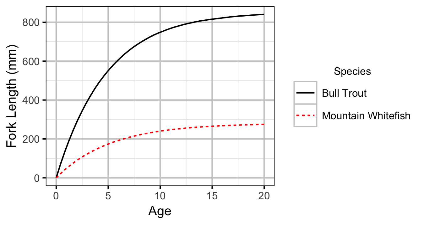
Bull Trout
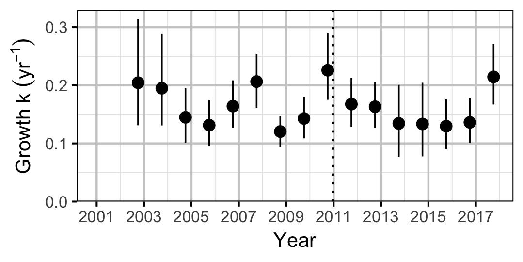
Mountain Whitefish
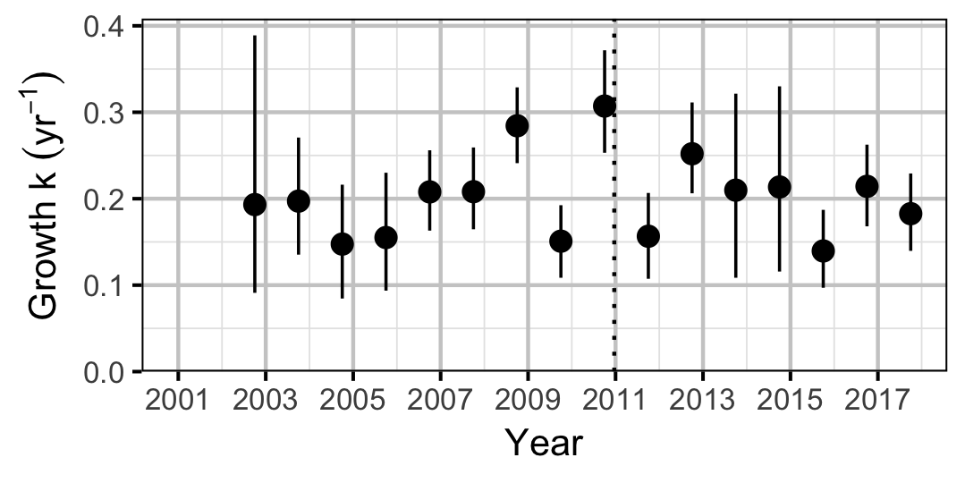
Condition
Bull Trout
Juvenile
Adult
Mountain Whitefish
Juvenile
Adult
Rainbow Trout
Juvenile
Adult
Largescale Sucker
Juvenile
Adult
Occupancy
Rainbow Trout
Burbot
Lake Whitefish
Northern Pikeminnow
Redside Shiner
Sculpins
Species Richness
Count
Rainbow Trout
Burbot
Northern Pikeminnow
Suckers
Movement
Bull Trout
Mountain Whitefish
Rainbow Trout
Largescale Sucker
Observer Length Correction
Abundance


Bull Trout
Juvenile
Adult
Mountain Whitefish
Juvenile
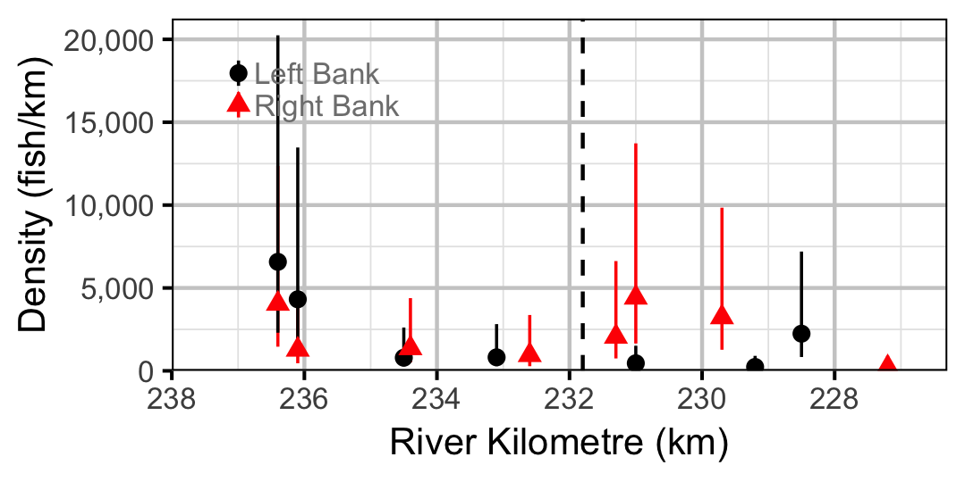
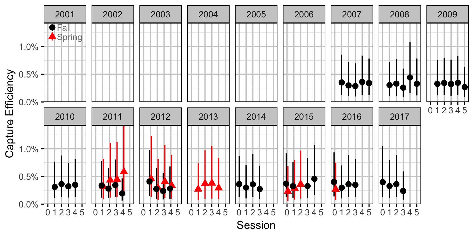
Adult
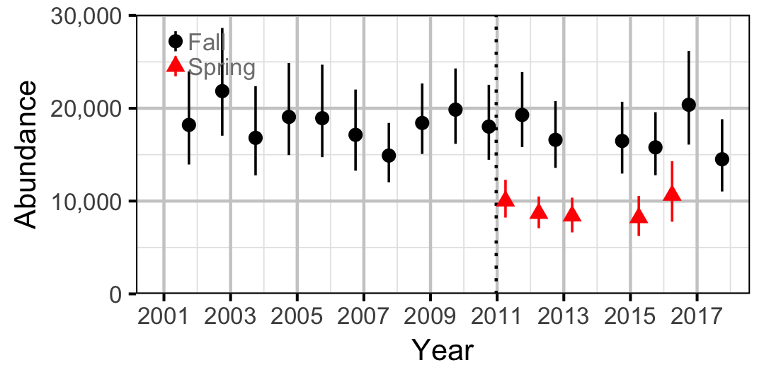
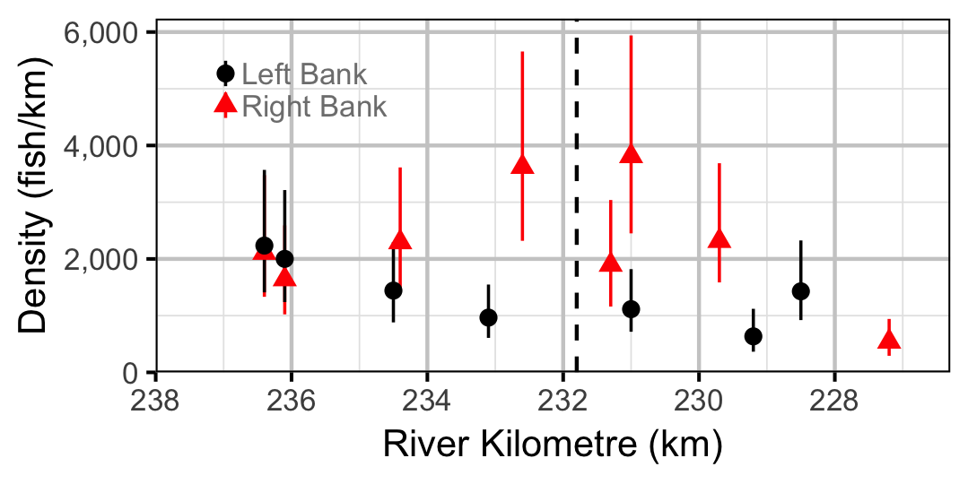
Rainbow Trout
Adult
Largescale Sucker
Adult
Species Diversity (Evenness)
Distribution
Bull Trout
Juvenile
Adult
Mountain Whitefish
Adult
Rainbow Trout
Burbot
Northern Pikeminnow
Suckers
Capture Effect
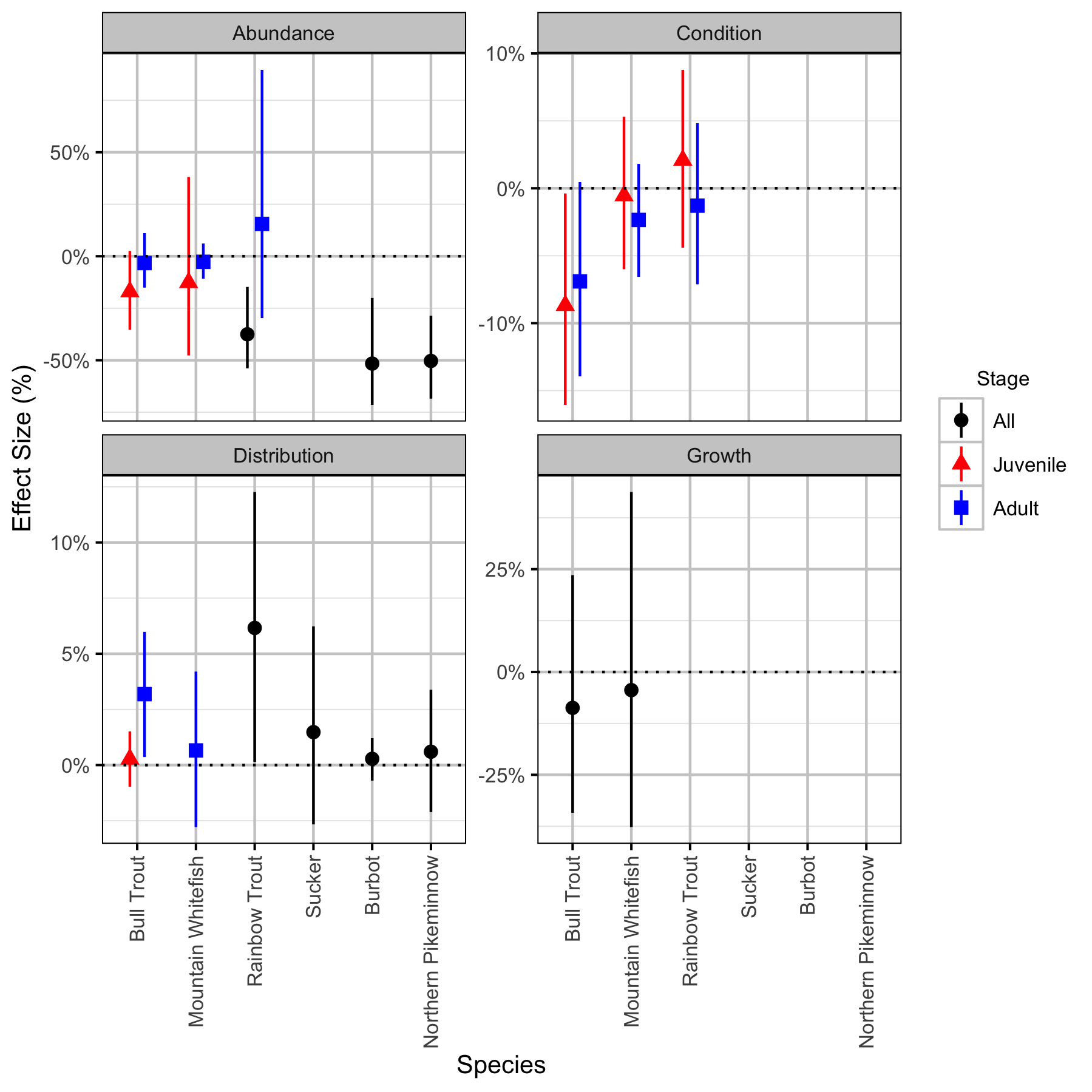
Effect Size
Significance
Table 82. The significance levels for the management hypotheses tested in the analyses. The Direction column indicates whether significant changes were positive or negative. The estimates and 95% lower and upper credible intervals are the effect sizes.
| Analysis | Species | Stage | Significance | Direction | Estimate | Lower | Upper |
|---|---|---|---|---|---|---|---|
| Abundance | Bull Trout | Juvenile | 0.0760 | -17 % | -35 % | 3 % | |
| Abundance | Bull Trout | Adult | 0.6053 | -3 % | -15 % | 11 % | |
| Abundance | Mountain Whitefish | Juvenile | 0.5307 | -13 % | -48 % | 38 % | |
| Abundance | Mountain Whitefish | Adult | 0.5253 | -3 % | -11 % | 6 % | |
| Abundance | Rainbow Trout | All | 0.0067 | - | -38 % | -54 % | -15 % |
| Abundance | Rainbow Trout | Adult | 0.5187 | 16 % | -30 % | 90 % | |
| Abundance | Burbot | All | 0.0027 | - | -52 % | -71 % | -20 % |
| Abundance | Northern Pikeminnow | All | 0.0007 | - | -50 % | -68 % | -29 % |
| Condition | Bull Trout | Juvenile | 0.0440 | - | -9 % | -16 % | 0 % |
| Condition | Bull Trout | Adult | 0.0667 | -7 % | -14 % | 0 % | |
| Condition | Mountain Whitefish | Juvenile | 0.8440 | -1 % | -6 % | 5 % | |
| Condition | Mountain Whitefish | Adult | 0.2547 | -2 % | -7 % | 2 % | |
| Condition | Rainbow Trout | Juvenile | 0.5227 | 2 % | -4 % | 9 % | |
| Condition | Rainbow Trout | Adult | 0.6573 | -1 % | -7 % | 5 % | |
| Distribution | Bull Trout | Juvenile | 0.6467 | 0 % | -1 % | 2 % | |
| Distribution | Bull Trout | Adult | 0.0187 | + | 3 % | 0 % | 6 % |
| Distribution | Mountain Whitefish | Adult | 0.6773 | 1 % | -3 % | 4 % | |
| Distribution | Rainbow Trout | All | 0.0467 | + | 6 % | 0 % | 12 % |
| Distribution | Sucker | All | 0.4880 | 1 % | -3 % | 6 % | |
| Distribution | Burbot | All | 0.5213 | 0 % | -1 % | 1 % | |
| Distribution | Northern Pikeminnow | All | 0.6720 | 1 % | -2 % | 3 % | |
| Growth | Bull Trout | All | 0.5213 | -9 % | -34 % | 24 % | |
| Growth | Mountain Whitefish | All | 0.8000 | -4 % | -38 % | 44 % |
Acknowledgements
The organisations and individuals whose contributions have made this analysis report possible include:
- BC Hydro
- Guy Martel
- Karen Bray
- Jason Watson
- Okanagan National Alliance
- Bronwen Lewis
- Amy Duncan
- Michael Zimmer
- Charlotte Whitney
- Golder Associates
- David Roscoe
- Dustin Ford
- Sima Usvyatsov
- Dana Schmidt
References
Bradford, Michael J, Josh Korman, and Paul S Higgins. 2005. “Using Confidence Intervals to Estimate the Response of Salmon Populations (Oncorhynchus Spp.) to Experimental Habitat Alterations.” Canadian Journal of Fisheries and Aquatic Sciences 62 (12): 2716–26. https://doi.org/10.1139/f05-179.
Carpenter, Bob, Andrew Gelman, Matthew D. Hoffman, Daniel Lee, Ben Goodrich, Michael Betancourt, Marcus Brubaker, Jiqiang Guo, Peter Li, and Allen Riddell. 2017. “Stan : A Probabilistic Programming Language.” Journal of Statistical Software 76 (1). https://doi.org/10.18637/jss.v076.i01.
Fabens, A J. 1965. “Properties and Fitting of the von Bertalanffy Growth Curve.” Growth 29 (3): 265–89.
He, Ji X., James R. Bence, James E. Johnson, David F. Clapp, and Mark P. Ebener. 2008. “Modeling Variation in Mass-Length Relations and Condition Indices of Lake Trout and Chinook Salmon in Lake Huron: A Hierarchical Bayesian Approach.” Transactions of the American Fisheries Society 137 (3): 801–17. https://doi.org/10.1577/T07-012.1.
Kery, Marc. 2010. Introduction to WinBUGS for Ecologists: A Bayesian Approach to Regression, ANOVA, Mixed Models and Related Analyses. Amsterdam; Boston: Elsevier. http://public.eblib.com/EBLPublic/PublicView.do?ptiID=629953.
Kery, Marc, and Michael Schaub. 2011. Bayesian Population Analysis Using WinBUGS : A Hierarchical Perspective. Boston: Academic Press. http://www.vogelwarte.ch/bpa.html.
Lin, J. 1991. “Divergence Measures Based on the Shannon Entropy.” IEEE Transactions on Information Theory 37 (1): 145–51. https://doi.org/10.1109/18.61115.
McElreath, Richard. 2016. Statistical Rethinking: A Bayesian Course with Examples in R and Stan. Chapman & Hall/CRC Texts in Statistical Science Series 122. Boca Raton: CRC Press/Taylor & Francis Group.
Plummer, Martyn. 2015. “JAGS Version 4.0.1 User Manual.” http://sourceforge.net/projects/mcmc-jags/files/Manuals/4.x/.
R Core Team. 2015. “R: A Language and Environment for Statistical Computing.” Vienna, Austria: R Foundation for Statistical Computing. http://www.R-project.org/.
von Bertalanffy, L. 1938. “A Quantitative Theory of Organic Growth (Inquiries on Growth Laws Ii).” Human Biology 10: 181–213.