Middle Columbia River Fish Indexing Analysis 2015
The suggested citation for this analytic report is:
Thorley, J.L. and Beliveau, A. (2016) Middle Columbia River Fish Indexing Analysis 2015. A Poisson Consulting Analysis Report. URL: https://www.poissonconsulting.ca/f/1492264933.
Background
The key management questions to be addressed by the analyses are:
- Is there a change in abundance of adult life stages of fish using the Middle Columbia River (MCR) that corresponds with the implementation of a year-round minimum flow?
- Is there a change in growth rate of adult life stages of the most common fish species using the MCR that corresponds with the implementation of a year-round minimum flow?
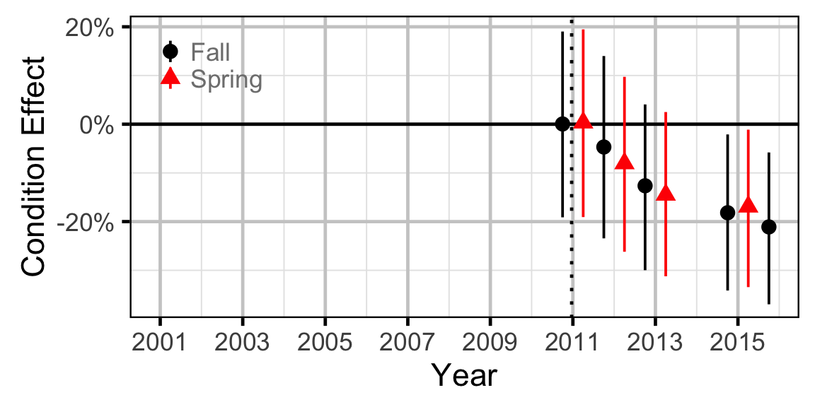
- Is there a change in body condition (measured as a function of relative weight to length) of adult life stages of fish using the MCR that corresponds with the implementation of a year-round minimum flow?
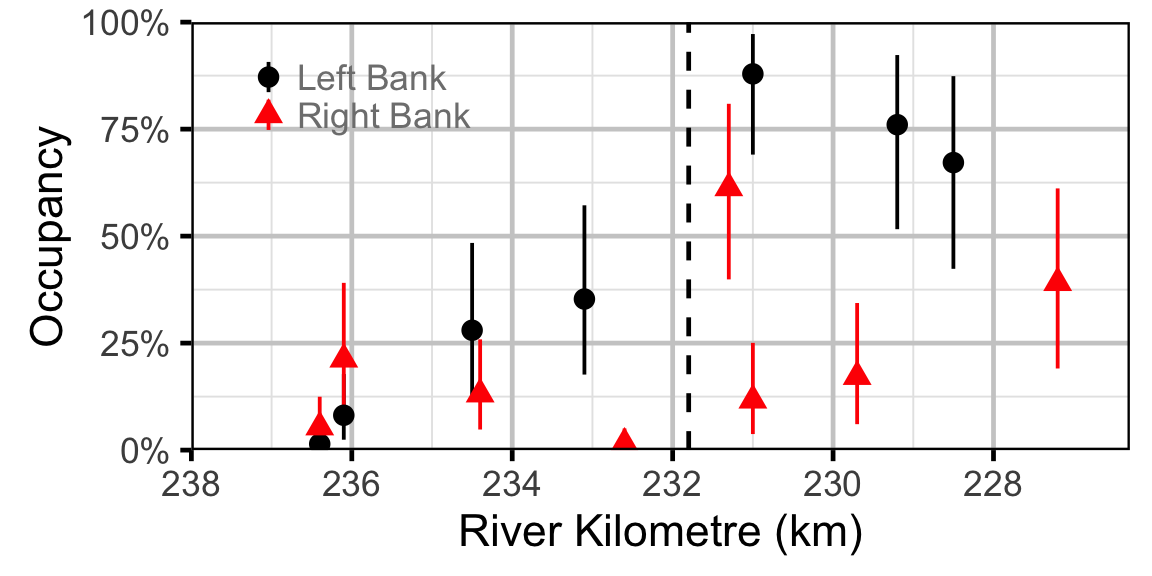
- Is there a change in spatial distribution of adult life stages of fish using the MCR that corresponds with the implementation of a year-round minimum flow?
Other objectives include the estimation of species richness, species diversity (evenness) and the modeling of environmental-fish metric relationships and scale age data. The year-round minimum flow was implemented in the winter of 2010 at the same time that a fifth turbine was added.
Methods
Data Preparation
The data were provided by Golder Associates.
Life-Stage
The four primary fish species were categorized as fry, juvenile or adult based on their lengths.
| Species | Fry | Juvenile |
|---|---|---|
| Bull Trout | <120 | <400 |
| Mountain Whitefish | <120 | <175 |
| Rainbow Trout | <120 | <250 |
| Largescale Sucker | <120 | <350 |
Statistical Analysis
Hierarchical Bayesian models were fitted to the count data using R version 3.3.0 (Team 2013) and JAGS 4.1.0 (Plummer 2015) which interfaced with each other via jaggernaut 2.3.3 (Thorley 2013). For additional information on hierarchical Bayesian modelling in the BUGS language, of which JAGS uses a dialect, the reader is referred to Kery and Schaub (2011, 41–44).
Unless specified, the models assumed vague (low information) prior distributions (Kery and Schaub 2011, 36). The posterior distributions were estimated from a minimum of 1,000 Markov Chain Monte Carlo (MCMC) samples thinned from the second halves of three chains of at least 10,000 iterations in length (Kery and Schaub 2011, 38–40). Model convergence was confirmed by ensuring that Rhat (Kery and Schaub 2011, 40) was less than 1.1 for each of the parameters in the model (Kery and Schaub 2011, 61). Model adequacy was confirmed by examination of residual plots.
The posterior distributions of the fixed (Kery and Schaub 2011, 75) parameters are summarised in terms of a point estimate (mean), lower and upper 95% credible limits (2.5th and 97.5th percentiles), the standard deviation (SD), percent relative error (half the 95% credible interval as a percent of the point estimate) and significance (Kery and Schaub 2011, 37, 42).
Variable selection was achieved by dropping insignificant (Kery and Schaub 2011, 37, 42) fixed (Kery and Schaub 2011, 77–82) variables and uninformative random variables. A fixed variables was considered to be insignificant if its significance was \(\geq\) 0.05 while a random variable was considered to be uninformative if its percent relative error was \(\geq\) 80%.
The results are displayed graphically by plotting the modeled relationships between particular variables and the response with 95% credible intervals (CRIs) with the remaining variables held constant. In general, continuous and discrete fixed variables are held constant at their mean and first level values respectively while random variables are held constant at their typical values (expected values of the underlying hyperdistributions) (Kery and Schaub 2011, 77–82). Where informative the influence of particular variables is expressed in terms of the effect size (i.e., percent change in the response variable) with 95% CRIs (Bradford, Korman, and Higgins 2005).
Growth
Annual growth was estimated from the inter-annual recaptures using the Fabens method (Fabens 1965) for estimating the von Bertalanffy (VB) growth curve (von Bertalanffy 1938). The VB curves is based on the premise that
\[ \frac{dl}{dt} = k (L_{\infty} - l)\]
where \(l\) is the length of the individual, \(k\) is the growth coefficient and \(L_{\infty}\) is the mean maximum length.
Integrating the above equation gives
\[ l_t = L_{\infty} (1 - e^{-k(t - t0)})\]
where \(l_t\) is the length at time \(t\) and \(t0\) is the time at which the individual would have had no length.
The Fabens form allows
\[ l_r = l_c + (L_{\infty} - l_c) (1 - e^{-kT})\]
where \(l_r\) is the length at recapture, \(l_c\) is the length at capture and \(T\) is the time at large.
Key assumptions of the growth model include:
- \(L_{\infty}\) is constant.
- \(k\) can vary with discharge regime.
- \(k\) can vary randomly with year.
- The residual variation in growth is independently and identically normally distributed.
Condition
Condition was estimated via an analysis of mass-length relations (He et al. 2008).
More specifically the model was based on the allometric relationship
\[ W = \alpha L^{\beta}\]
where \(W\) is the weight (mass), \(\alpha\) is the coefficent, \(\beta\) is the exponent and \(L\) is the length.
To improve chain mixing the relation was log-transformed, i.e.,
\[ \log(W) = \log(\alpha) + \beta \log(L)\]
and the logged lengths centered, i.e., \(\log(L) - \overline{\log(L)}\), prior to model fitting.
Preliminary analyses indicated that the variation in the exponent \(\beta\) with respect to year was not informative.
Key assumptions of the final condition model include:
- The expected weight varies with length as an allometric relationship.
- The intercept of the log-transformed allometric relationship is described by a linear mixed model.
- The intercept of the log-transformed allometric relationship varies with discharge regime and season.
- The intercept of the log-transformed allometric relationship varies randomly with year, site and the interaction between year and site.
- The slope of the log-transformed allometric relationship is described by a linear mixed model.
- The slope of the log-transformed allometric relationship varies with discharge regime and season.
- The slope of the log-transformed allometric relationship varies randomly with year.
- The residual variation in weight for the log-transformed allometric relationship is independently and identically normally distributed.
Occupancy
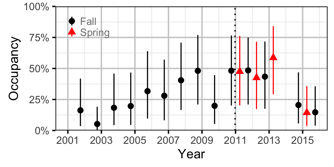
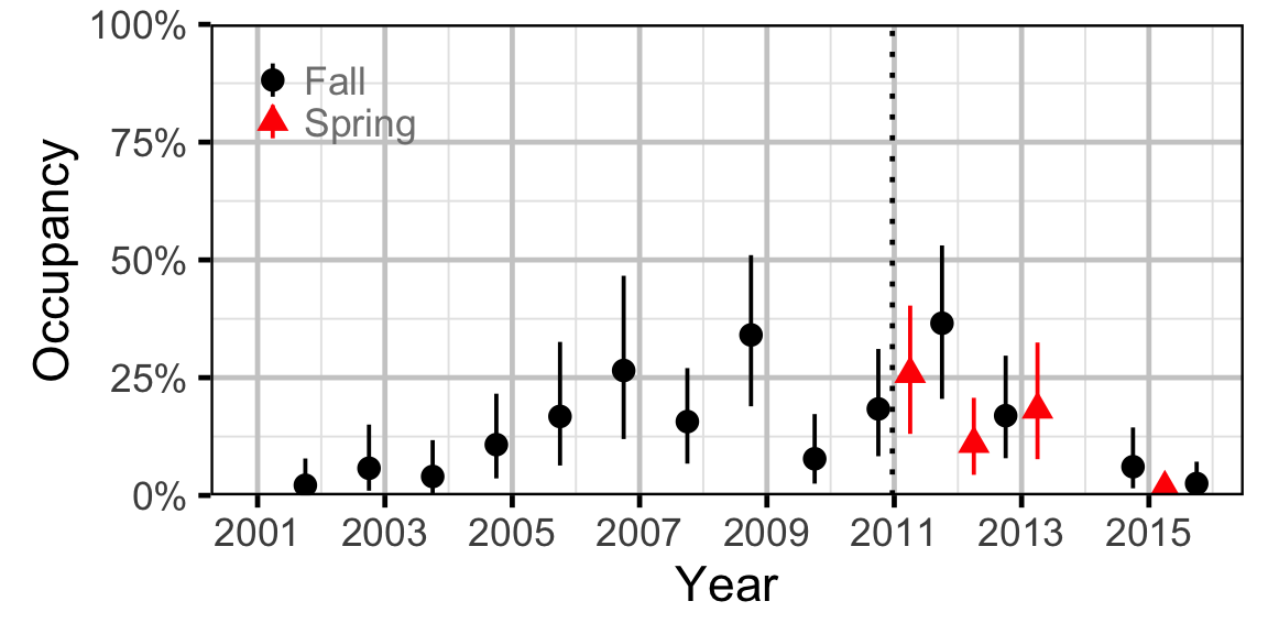
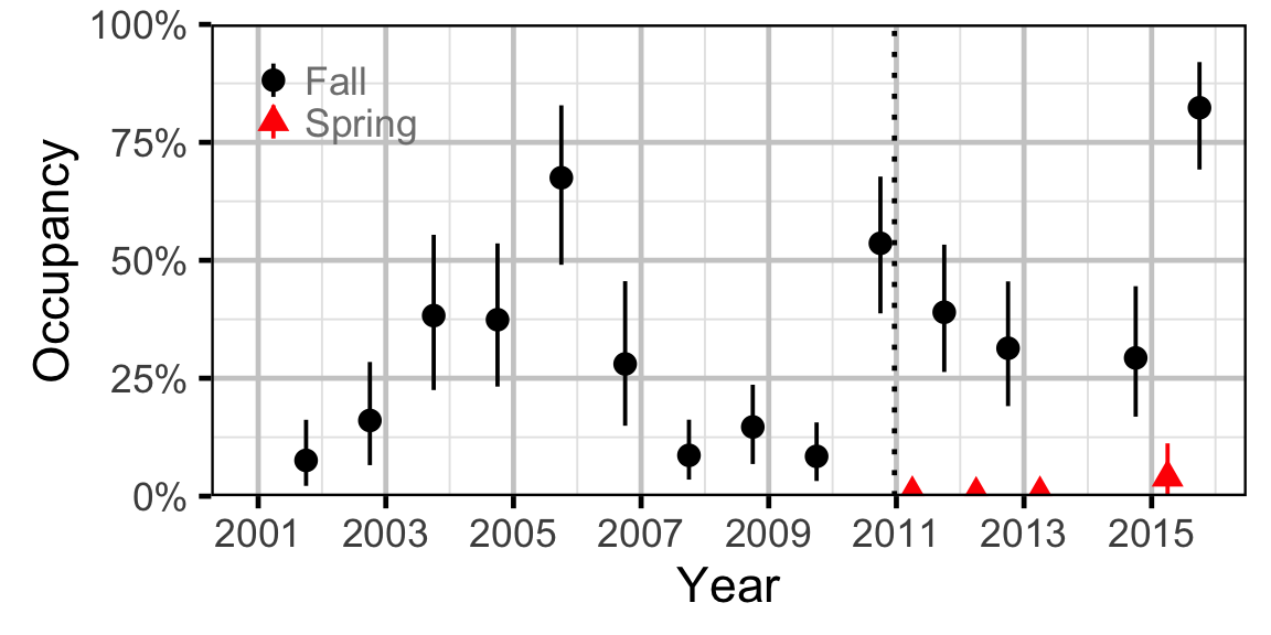
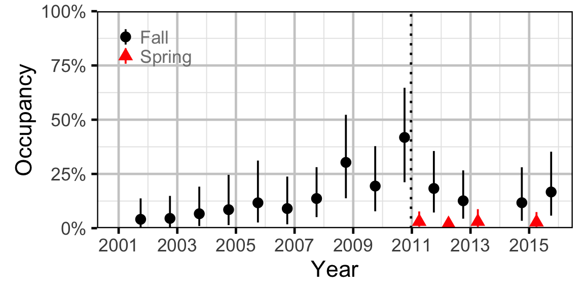
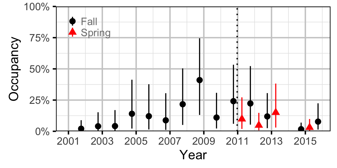
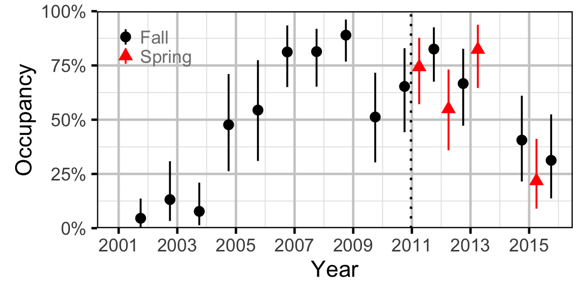
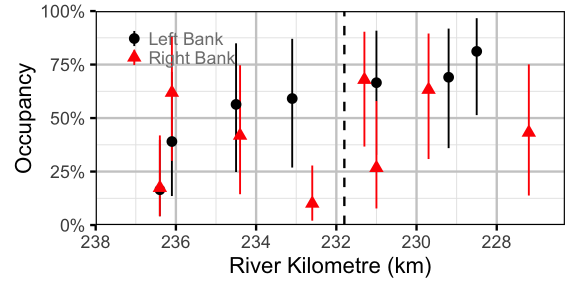
Occupancy, which is the probability that a particular species was present at a site, was estimated from the temporal replication of detection data (Kery, 2010; Kery and Schaub, 2011, pp. 238-242 and 414-418), i.e., each site was surveyed multiple times within a season. A species was considered to have been detected if one or more individuals of the species were caught or counted. It is important to note that the model estimates the probability that the species was present at a given (or typical) site in a given (or typical) year as opposed to the probability that the species was present in the entire study area. We focused on Northern Pikeminnow, Burbot, Lake Whitefish, Rainbow Trout, Redside Shiner and Sculpins because they were low enough density to not to be present at all sites at all times yet were encounted sufficiently often to provide information on spatial and temporal changes.
Key assumptions of the occupancy model include:
- Occupancy (probability of presence) is described by a generalized linear mixed model with a logit link.
- Occupancy varies with discharge regime and season.
- Occupancy varies randomly with site and year.
- Sites are closed, i.e., the species is present or absent at a site for all the sessions in a particular season of a year.
- Observed presence is described by a bernoulli distribution, given occupancy.
Species Richness
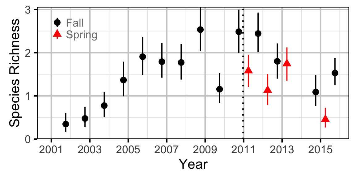
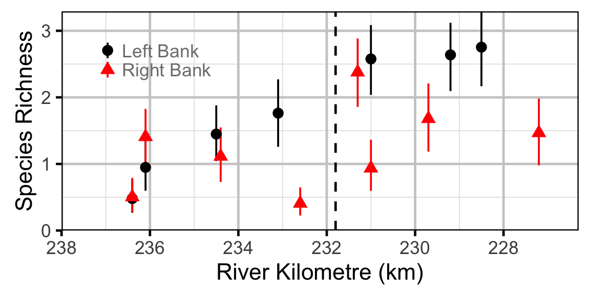
The estimated probabilities of presence for the six species considered in the occupany analyses were summed to give the expected species richnesses at a given (or typical) site in a given (or typical) year.
Count
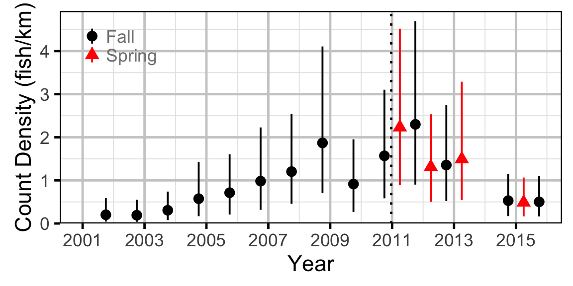
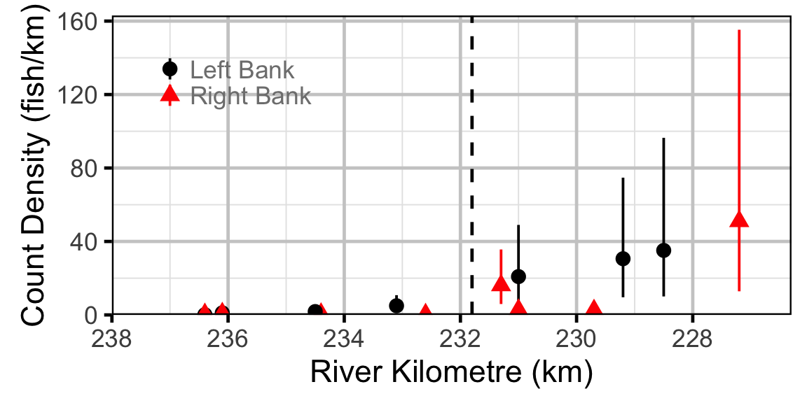
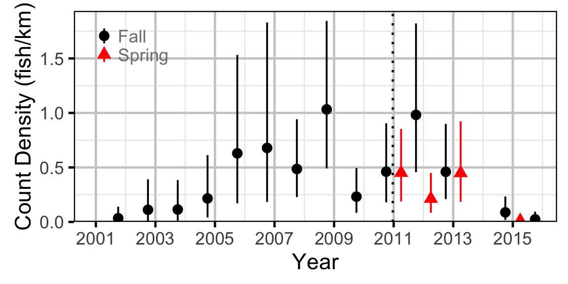
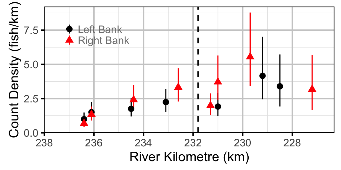
The count data were analysed using an overdispersed Poisson model (Kery, 2010; Kery and Schaub, 2011, pp. 168-170,180 and 55-56) to provide estimates of the lineal river count density (count/km) by year and site. Unlike Kery (2010) and Kery and Schaub (2011), which used a log-normal distribution to account for the extra-Poisson variation, the current model used a gamma distribution with identical shape and scale parameters because it has a mean of 1 and therefore no overall effect on the expected count. The count data does not enable us to estimate abundance nor observer efficiency, but it enables us to estimate an expected count, which is the product of the two. As such it is necessary to assume that changes in observer efficiency are negligible in order to interpret the estimates as relative density.
Key assumptions of the abundance model include:
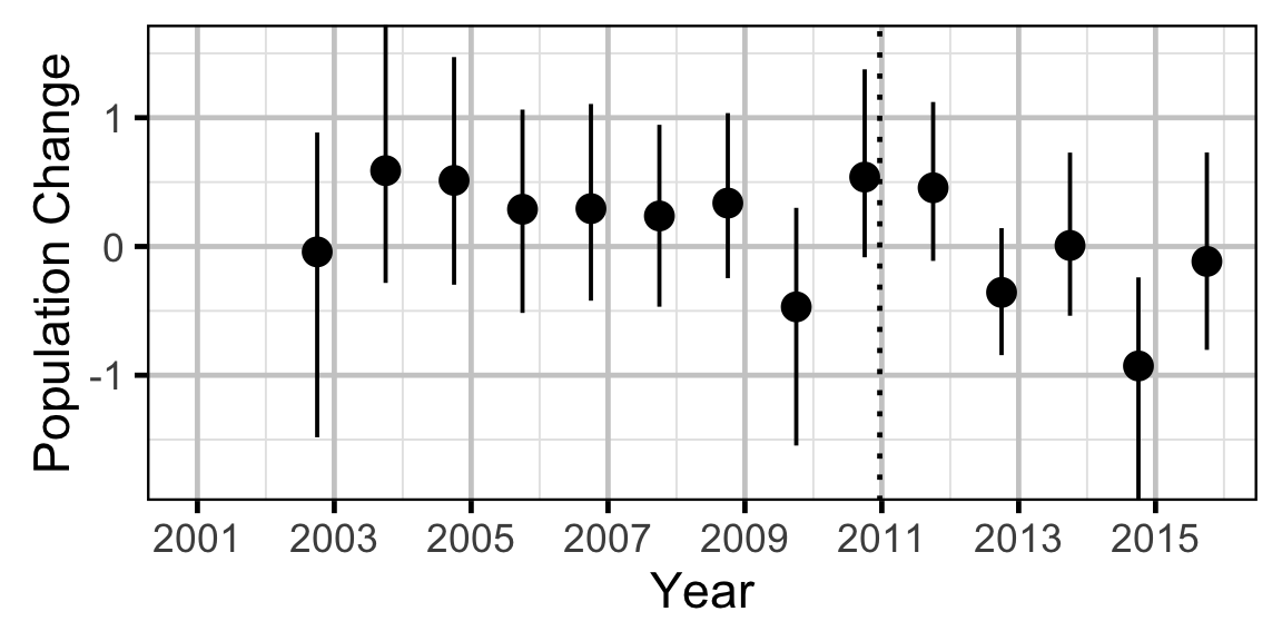
- Lineal density (fish/km) is described by an autoregressive generalized linear mixed model with a logarithm link.
- Lineal density (fish/km) varies with season.
- Lineal density (fish/km) varies randomly with year, river kilometer, site and the interaction between site and year.
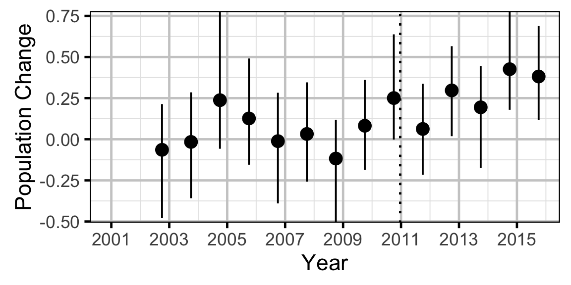
- The effect of year on lineal density (fish/km) is autoregressive with a lag of one year and varies with discharge regime.
- The regression coefficient of river kilometre is described by a linear mixed model.
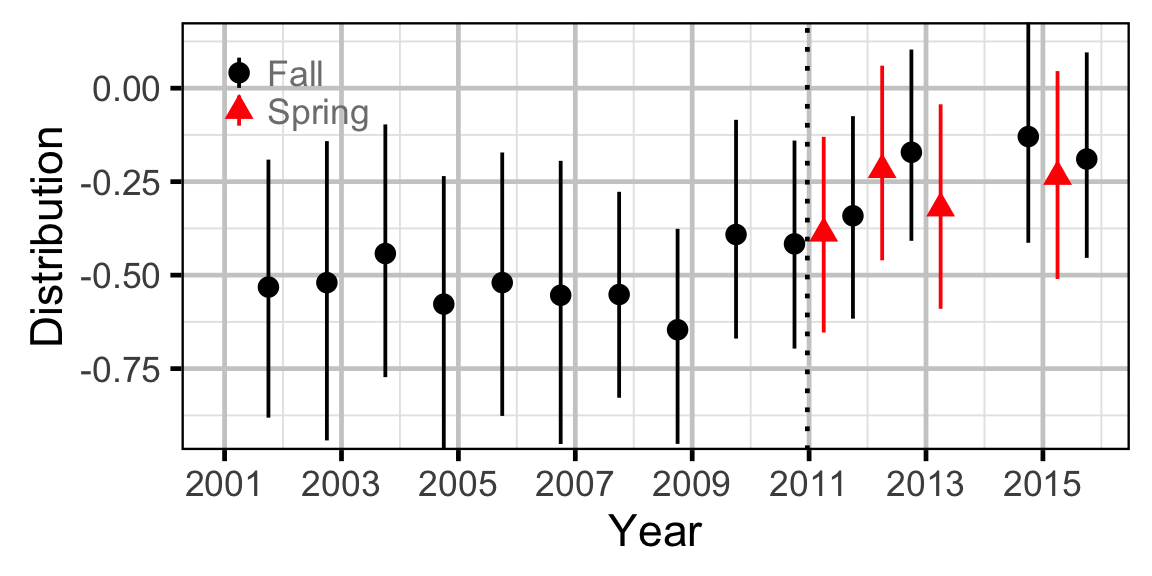
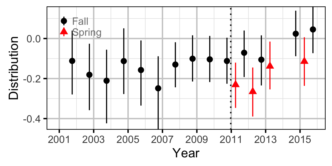
- The effect of river kilometre on lineal density (distribution of density along the river) varies with discharge regime and season.
- The effect of river kilometre on lineal density (distribution of density along the river) varies randomly with year.
- The counts are gamma-Poisson distributed, given the mean count.
Movement
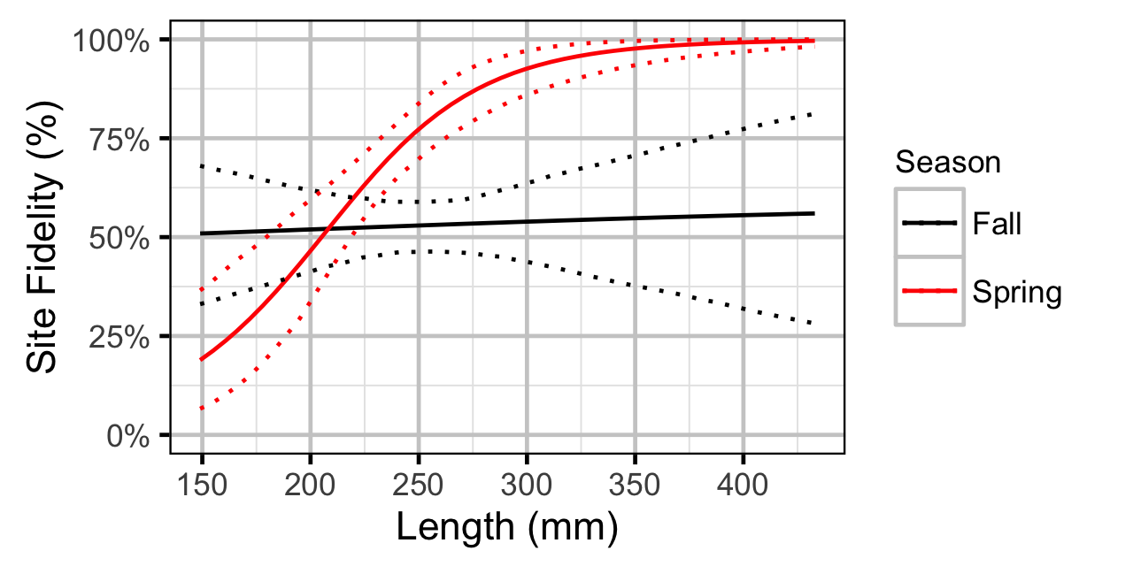
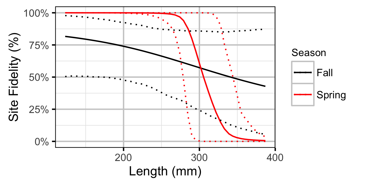
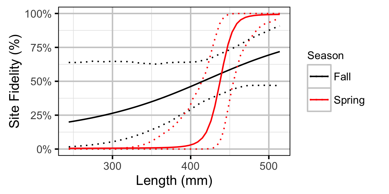
The extent to which sites are closed, i.e., fish remain at the same site between sessions, was evaluated from a logistic ANCOVA (Kery 2010). The model estimated the probability that intra-annual recaptures were caught at the same site versus a different one.
Key assumptions of the site fidelity model include:
- Site fidelity varies with season, length and the interaction between season and length.
- Observed site fidelity is Bernoulli distributed.
Observer Length Correction
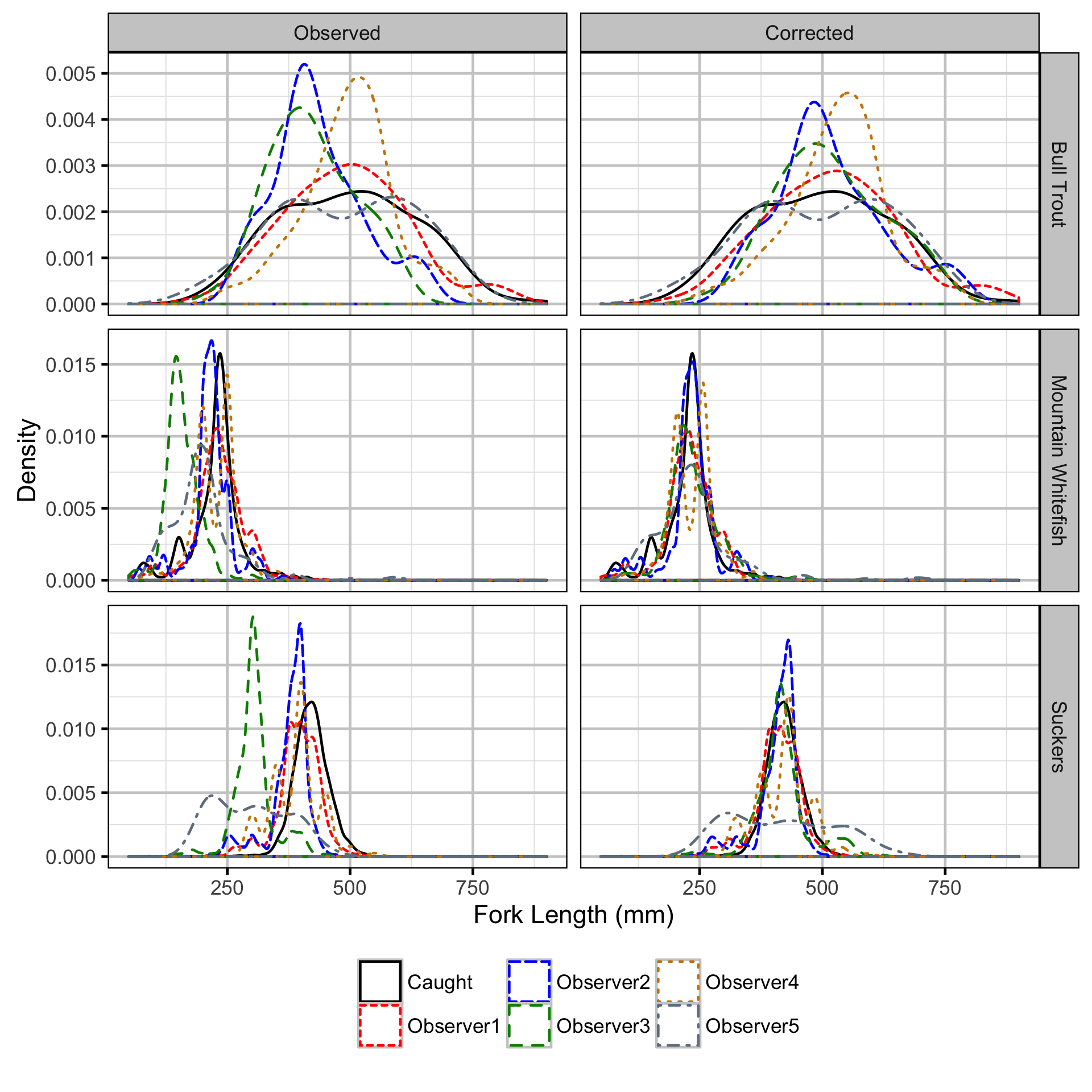
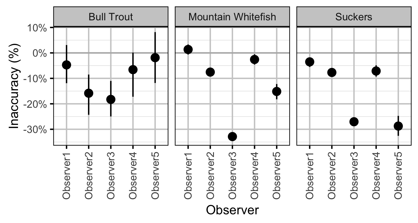
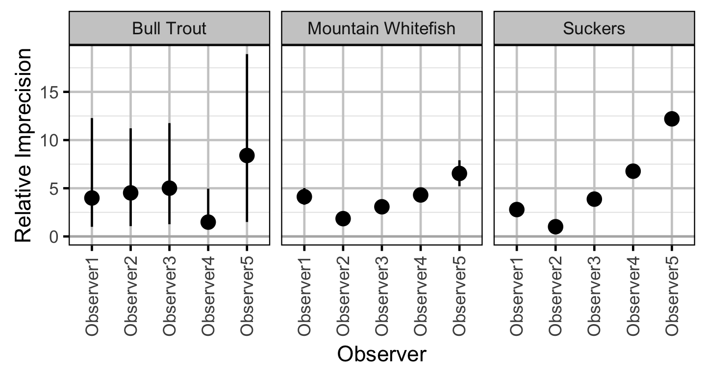
The bias (accuracy) and error (precisions) in observer’s fish length estimates were quantified using a model with a categorical distribution that compared the proportions of fish in different length-classes for each observer to the equivalent proportions for the measured fish.
Key assumptions of the observer length correction model include:
- The expected length bias can vary by observer.
- The expected length error can vary by observer.
- The residual variation in length is independently and identically normally distributed.
The observed fish lengths were corrected for the estimated length biases.
Abundance
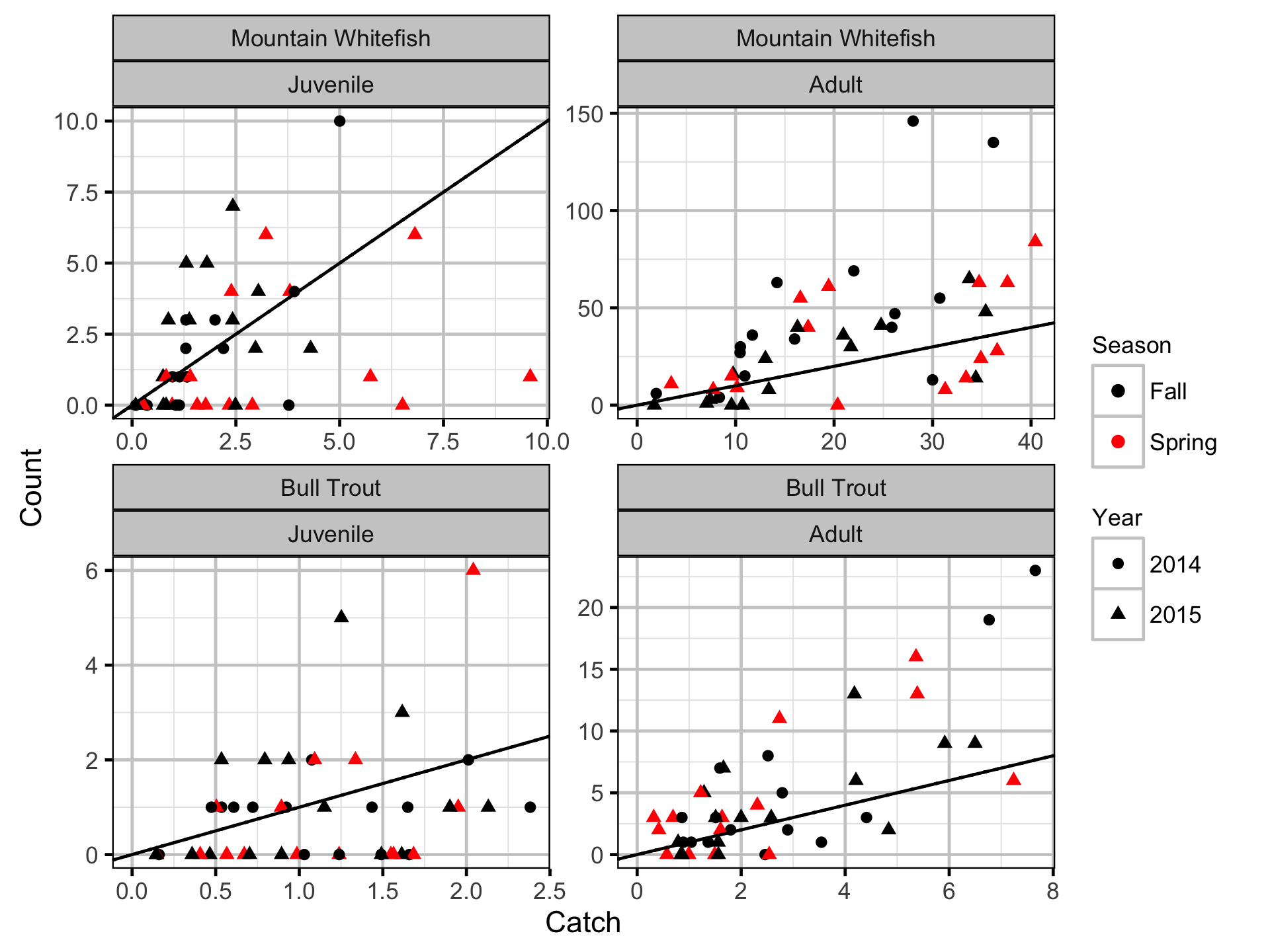
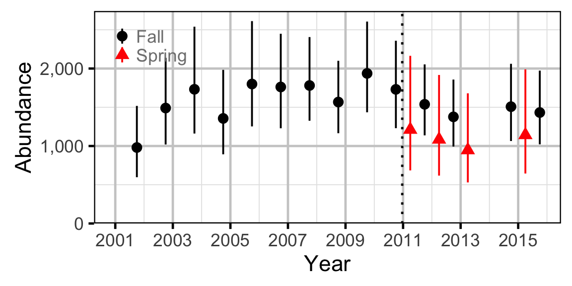
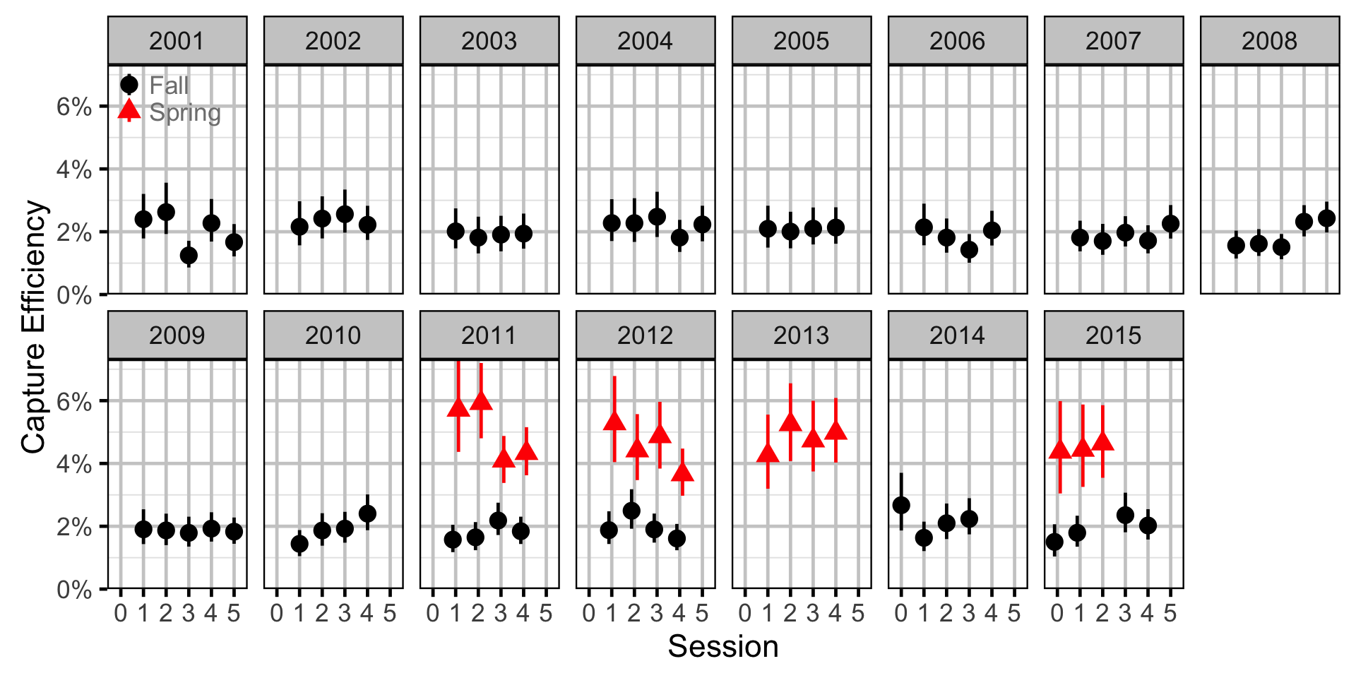
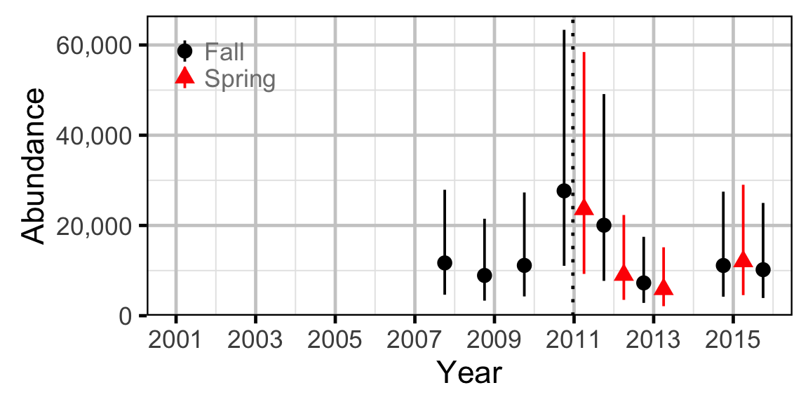
The catch data were analysed using a capture-recapture-based overdispersed Poisson model to provide estimates of capture efficiency and absolute abundance. To maximize the number of recaptures the model grouped all the sites into a supersite for the purposes of estimating the number of marked fish but analysed the total captures at the site level.
Key assumptions of the abundance model include:
- Lineal density (fish/km) varies with year, season and river km.
- Lineal density (fish/km) varies randomly with site and the interaction between site and year.
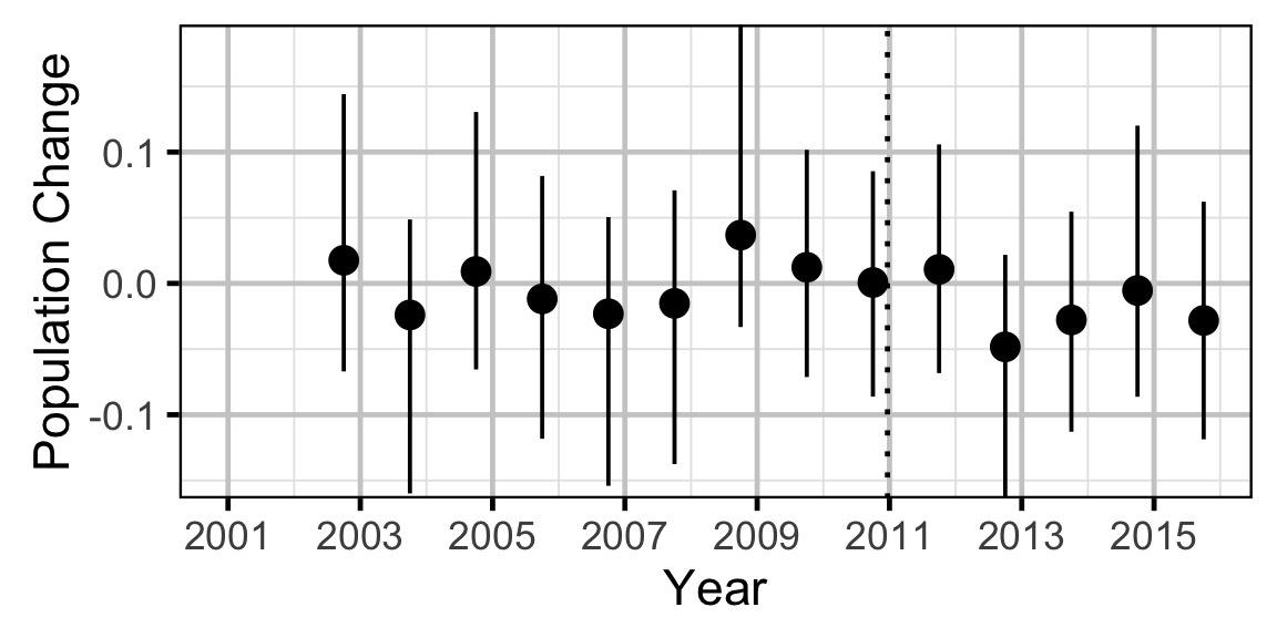
- The effect of year on lineal density (fish/km) is autoregressive with a lag of one year and varies with discharge regime.
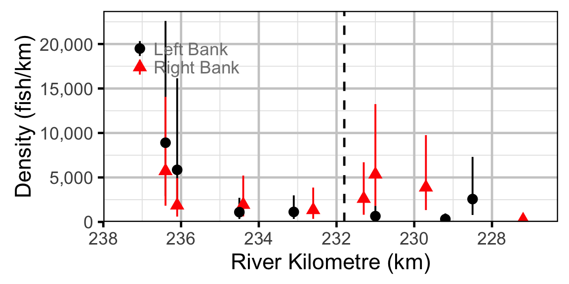
- The effect of river km on lineal density (fish/km) (distribution) varies with discharge regime and season.
- The effect of river km on lineal density (fish/km) (distribution) varies randomly with year.
- Efficiency (probability of capture) varies by season and method (capture versus count).
- Efficiency varies randomly by session within season within year.
- Marked and unmarked fish have the same probability of capture.
- There is no tag loss, migration (at the supersite level), mortality or misidentification of fish.
- The number of fish caught is gamma-Poisson distributed.
Note that the analysis did not converge for Largescale Suckers. Excluding the 2001 data from the analysis (there was no data for this species from 2002 to 2009) did not improve convergence.
Species Evenness
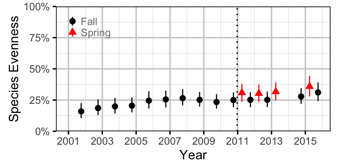
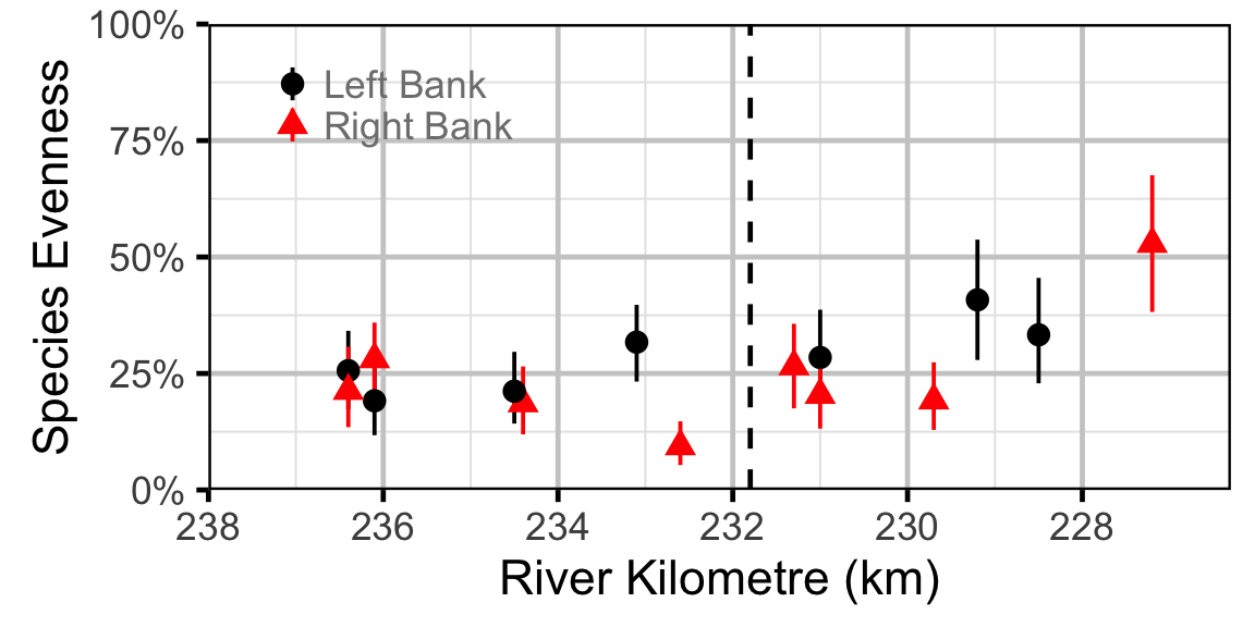
The site and year estimates of the lineal bank count densities from the count model for Rainbow Trout, Suckers, Burbot and Northern Pikeminnow were combined with the equivalent count estimates for Bull Trout and Adult Mountain Whitefish from the abundance model to calculate the shannon index of evenness \((E)\). The index was calculated using the following formula where \(S\) is the number of species and \(p_i\) is the proportion of the total count belonging to the ith species.
\[ E = \frac{-\sum p_i \log(p_i)}{\log(S)}\]
Long-Term Trends
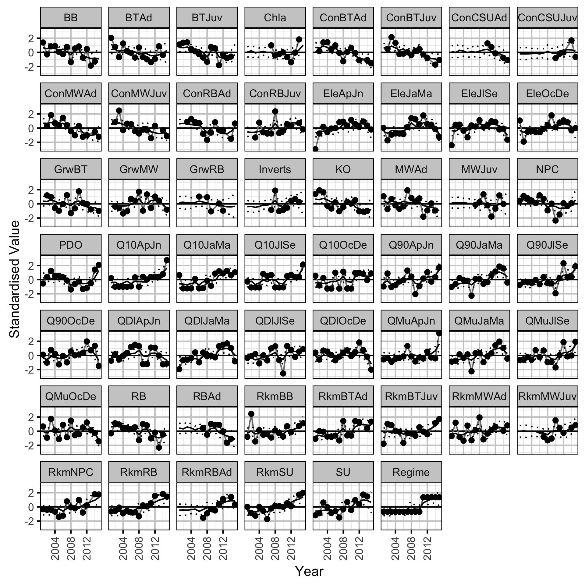
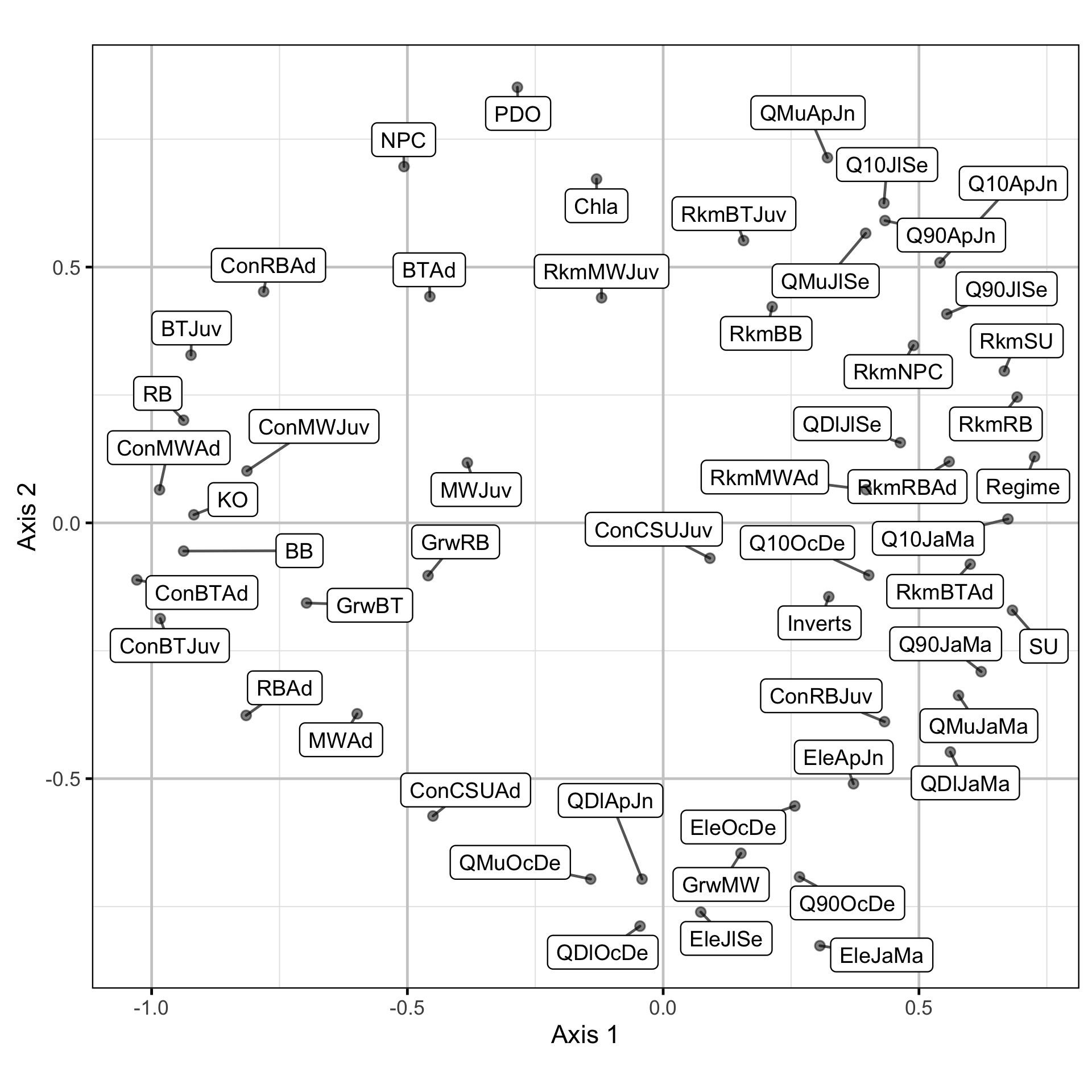
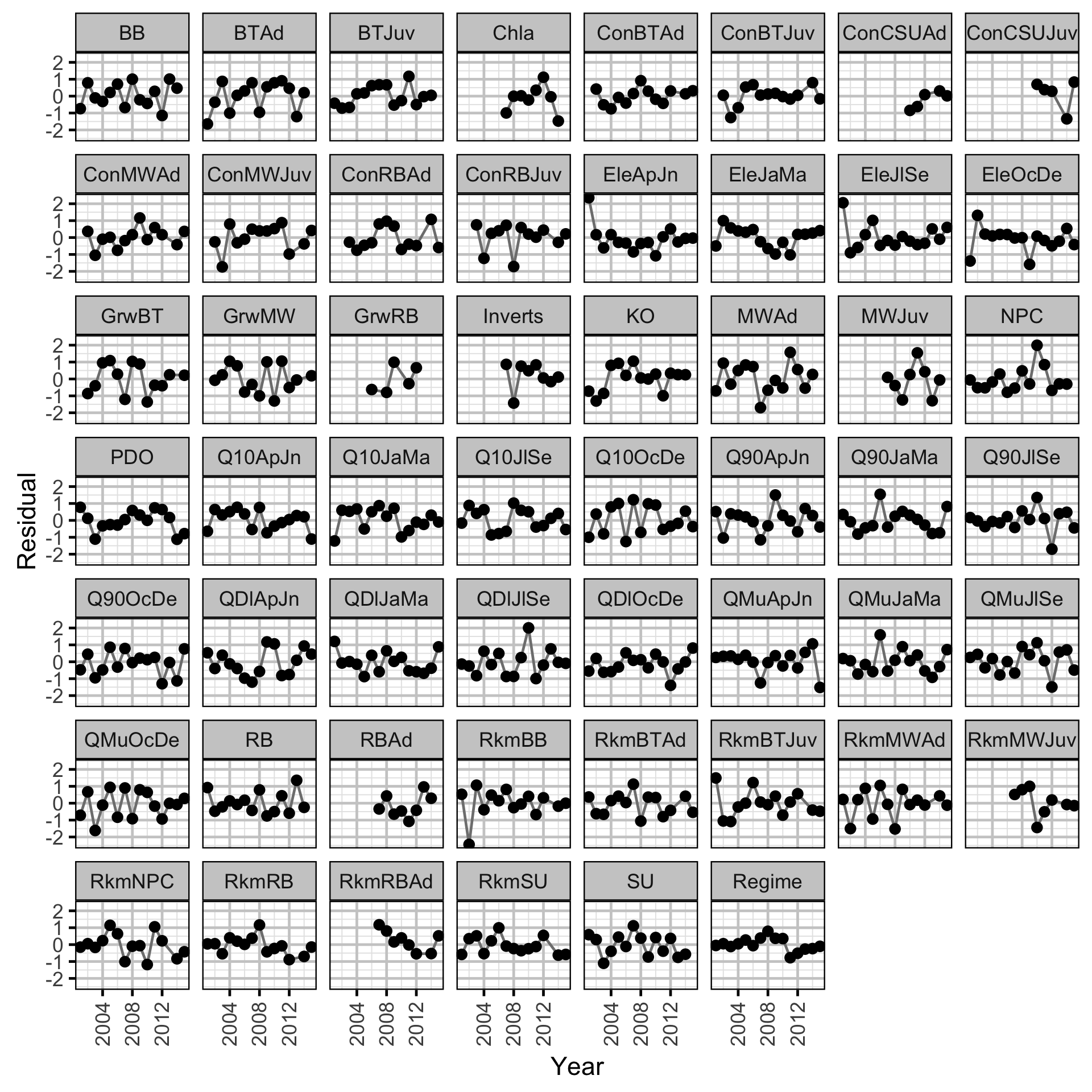
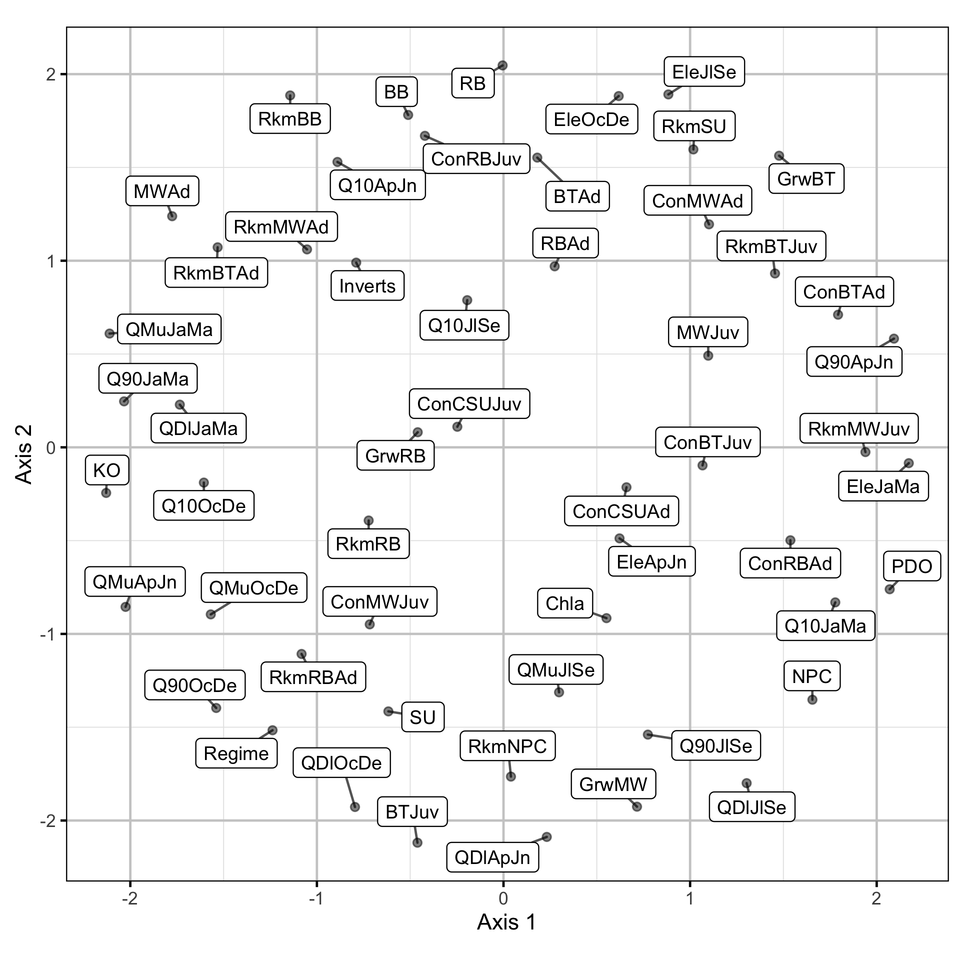
The long-term congruence between the yearly fall fish metrics (Grw = Estimated growth \(k\), Con = Estimated condition effect, Blank = Estimated population growth rate, Rkm = Estimated effect of centred river kilometre on log density) by life stage (Juv = Juvenile, AD = Adult) and a range of environmental variables including the tri-monthly (JaMa = January - March, ApJn = April - June, JlSe = July - September, OcDe = October - December) discharge from Revelstoke Dam (Q10, QMu = Mean, Q90, QDlt = Mean absolute difference) and the elevation (Ele), the Pacific Decadal Oscillation (PDO), the chlorophyll-a (ChlA) and invertebrate production (Inv) and the kokanee abundance (KO) was examined using Dynamic Factor Analysis (Zuur, Tuck, and Bailey 2003). Due to the rotation problem the underlying trends were indeterminate (Abmann, Boysen-Hogrefe, and Pape 2014). The October to December discharge and elevation values were lead (opposite of lagged) by one year to account for the fact that they occurred after sampling.
Key assumptions of the Dynamic Factor Analysis (DFA) model include:
- The time series are described by three underlying trends.
- The random walk processes in the trends are normally distributed.
- The residual variation in the standardised variables is normally distributed.
The similarities were represented visually by using non-metric multidimensional scaling (NMDS) to map the distances onto two-dimensional space. The more similar two time series are the closer they will tend to be in the resultant NMDS plot.
Short-Term Correlations
To assess the short-term congruence between the yearly fish metrics and the environmental variables, the pair-wise distances between the residuals from the DFA model were calculated as \(1 - abs(cor(x, y))\) where \(cor\) is the Pearson correlation, \(abs\) the absolute value and \(x\) and \(y\) are the two time series being compared.
The short-term similarities were represented visually by using NMDS to map the distances onto two-dimensional space.
Scale Age
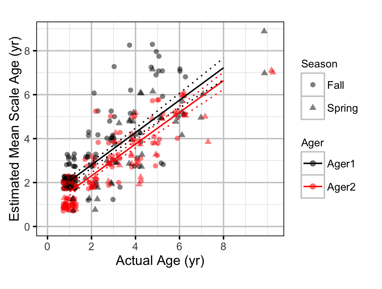
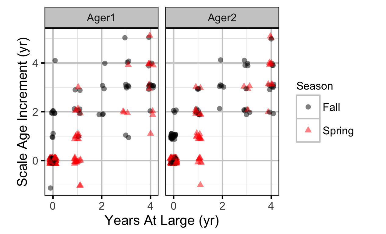
The age of Mountain Whitefish was estimated from scales by two independent agers. The scale aging process was repeated twice per ager, leading to two observations per ager per fish encounter (Hurlbert 1984). The actual age was determined from the length of each fish at first capture based on the stage cutoffs by season. The scale ages were analysed using a linear mixed model.
Key assumptions of the scale age model include:
- The scale age varies by ager.
- The scale age varies randomly with fish encounter and ager within fish encounter.
- The scale age varies linearly with age.
- The effect of age on scale age varies by ager.
- The random effects are normally distributed.
- The residual variation in the scale ages (replicate within ager within encounter) is described by a zero-truncated normal distribution.
Model Code
The JAGS model code, which uses a series of naming conventions, is presented below.
Growth
| Variable/Parameter | Description |
|---|---|
bK[i] |
Expected growth coefficient in the ith year |
bKIntercept |
Intercept for log(bK) |
bKRegime[i] |
Effect of ith regime on log(bK) |
bKYear[i] |
Random effect of ith Year on log(bK) |
bLinf |
Mean maximum length |
eGrowth[i] |
Expected Growth of the ith recapture |
Growth[i] |
Change in length of the ith fish between release and recapture |
LengthAtRelease[i] |
Length of the ith recapture when released |
nRegime[i] |
Number of regimes |
sGrowth |
SD of residual variation in Growth |
sKYear[i] |
SD of effect of Year on log(bK) |
Threshold |
Last year of the first regime |
Year[i] |
Year the ith recapture was released |
Years[i] |
Number of years between release and recapture for the ith recapture |
Growth - Model1
model {

  bKIntercept ~ dnorm (0, 5^-2)

  bKRegime[1] <- 0
  for(i in 2:nRegime) {
    bKRegime[i] ~ dnorm(0, 5^-2)
  }

  sKYear ~ dunif (0, 5)
  for (i in 1:nYear) {
    bKYear[i] ~ dnorm(0, sKYear^-2)
    log(bK[i]) <- bKIntercept + bKRegime[step(i - Threshold) + 1] + bKYear[i]
  }

  bLinf ~ dunif(100, 1000)
  sGrowth ~ dunif(0, 100)

  for (i in 1:length(Year)) {

    eGrowth[i] <- (bLinf - LengthAtRelease[i]) * (1 - exp(-sum(bK[Year[i]:(Year[i] + Years[i] - 1)])))

    Growth[i] ~ dnorm(eGrowth[i], sGrowth^-2)
  }
  tGrowth <- bKRegime[2]
}
Condition
| Variable/Parameter | Description |
|---|---|
bWeightIntercept |
Intercept for eWeightIntercept |
bWeightRegimeIntercept[i] |
Effect of ith regime on bWeightIntercept |
bWeightRegimeSlope[i] |
Effect of ith regime on bWeightSlope |
bWeightSeasonIntercept[i] |
Effect of ith season on bWeightIntercept |
bWeightSeasonSlope[i] |
Effect of ith season on bWeightSlope |
bWeightSiteIntercept[i] |
Random effect of ith site on bWeightIntercept |
bWeightSiteYearIntercept[i,j] |
Random effect of ith site in jth year on bWeightIntercept |
bWeightSlope |
Intercept for eWeightSlope |
bWeightYearIntercept[i] |
Random effect of ith year on bWeightIntercept |
bWeightYearSlope[i] |
Random effect of ith year on bWeightSlope |
eWeight[i] |
Expected weight of the ith fish |
eWeightIntercept[i] |
Intercept for log(eWeight[i]) |
eWeightSlope[i] |
Slope for log(eWeight[i]) |
Length[i] |
Length of ith fish |
sWeight |
Residual SD of Weight |
sWeightSiteIntercept |
SD for the effect of site on bWeightIntercept |
sWeightSiteYearIntercept |
SD for the effect of the combination of site and year on eWeightIntercept |
sWeightYearIntercept |
SD of the effect of year on bWeightIntercept |
sWeightYearSlope |
SD for the random effect of year on eWeightSlope |
Weight[i] |
Weight of ith fish |
Condition - Model1
model {

  bWeightIntercept ~ dnorm(5, 5^-2)
  bWeightSlope ~ dnorm(3, 5^-2)

  bWeightRegimeIntercept[1] <- 0
  bWeightRegimeSlope[1] <- 0

  for(i in 2:nRegime) {
    bWeightRegimeIntercept[i] ~ dnorm(0, 5^-2)
    bWeightRegimeSlope[i] ~ dnorm(0, 5^-2)
  }

  bWeightSeasonIntercept[1] <- 0
  bWeightSeasonSlope[1] <- 0
  for(i in 2:nSeason) {
    bWeightSeasonIntercept[i] ~ dnorm(0, 5^-2)
    bWeightSeasonSlope[i] ~ dnorm(0, 5^-2)
  }

  sWeightYearIntercept ~ dunif(0, 5)
  sWeightYearSlope ~ dunif(0, 5)
  for(yr in 1:nYear) {
    bWeightYearIntercept[yr] ~ dnorm(0, sWeightYearIntercept^-2)
    bWeightYearSlope[yr] ~ dnorm(0, sWeightYearSlope^-2)
  }

  sWeightSiteIntercept ~ dunif(0, 5)
  sWeightSiteYearIntercept ~ dunif(0, 5)
  for(st in 1:nSite) {
    bWeightSiteIntercept[st] ~ dnorm(0, sWeightSiteIntercept^-2)
    for(yr in 1:nYear) {
      bWeightSiteYearIntercept[st, yr] ~ dnorm(0, sWeightSiteYearIntercept^-2)
    }
  }

  sWeight ~ dunif(0, 5)
  for(i in 1:length(Year)) {

    eWeightIntercept[i] <- bWeightIntercept
        + bWeightRegimeIntercept[Regime[i]]
        + bWeightSeasonIntercept[Season[i]]
        + bWeightYearIntercept[Year[i]]
        + bWeightSiteIntercept[Site[i]]
        + bWeightSiteYearIntercept[Site[i],Year[i]]

    eWeightSlope[i] <- bWeightSlope
        + bWeightRegimeSlope[Regime[i]]
        + bWeightSeasonSlope[Season[i]]
        + bWeightYearSlope[Year[i]]

    log(eWeight[i]) <- eWeightIntercept[i] + eWeightSlope[i] * Length[i]
    Weight[i] ~ dlnorm(log(eWeight[i]) , sWeight^-2)
  }
  tCondition1 <- bWeightRegimeIntercept[2]
  tCondition2 <- bWeightRegimeSlope[2]
}
Occupancy
| Variable/Parameter | Description |
|---|---|
bOccupancy |
Intercept of logit(eOccupancy) |
bOccupancyRegime[i] |
Effect of ith regime on logit(eOccupancy) |
bOccupancySeason[i] |
Effect of ith season on logit(eOccupancy) |
bOccupancySite[i] |
Effect of ith site on logit(eOccupancy) |
bOccupancyYear[i] |
Effect of ith year on logit(eOccupancy) |
eObserved[i] |
Probability of observing species on ith site visit |
eOccupancy[i] |
Predicted occupancy (species presence versus absence) on ith site visit |
nRegime |
Number of regimes in the dataset (2) |
nSeason |
Number of seasons in the dataset (2) |
nSite |
Number of sites in the dataset |
nYear |
Number of years of data |
Observed[i] |
Whether the species was observed on ith site visit (0 or 1) |
Regime[i] |
Regime ofith site visit |
Season[i] |
Season of ith site visit |
Site[i] |
Site of ith site visit |
sOccupancySite |
SD parameter for the distribution of bOccupancySite[i] |
sOccupancyYear |
SD parameter for the distribution of bOccupancyYear[i] |
Year[i] |
Year of ith site visit |
Occupancy - Model1
model {

  bOccupancy ~ dnorm(0, 5^-2)
  bOccupancySeason[1] <- 0
  for(i in 2:nSeason) {
    bOccupancySeason[i] ~ dnorm(0, 5^-2)
  }

  bOccupancyRegime[1] <- 0
  for(i in 2:nRegime) {
    bOccupancyRegime[i] ~ dnorm(0, 5^-2)
  }

  sOccupancyYear ~ dunif(0, 5)
  for (yr in 1:nYear) {
    bOccupancyYear[yr] ~ dnorm(0, sOccupancyYear^-2)
  }

  sOccupancySite ~ dunif(0, 5)
  for (st in 1:nSite) {
    bOccupancySite[st] ~ dnorm(0, sOccupancySite^-2)
  }
  for (i in 1:length(Year)) {
    logit(eOccupancy[i]) <- bOccupancy
    + bOccupancyRegime[Regime[i]] + bOccupancySeason[Season[i]]
    + bOccupancySite[Site[i]] + bOccupancyYear[Year[i]]
    eObserved[i] <- eOccupancy[i]
    Observed[i] ~ dbern(eObserved[i])
  }
}
Count
| Variable/Parameter | Description |
|---|---|
bDensitySeason[i] |
Effect of ith season on log(eDensity) |
bDensitySite[i] |
Effect of ith site on log(eDensity) |
bDensitySiteYear[i, j] |
Effect of ith site in jth year on log(eDensity) |
bDensityYear[i] |
Random effect of ith year on log(eDensity) |
bDistribution |
Intercept of eDistribution |
bDistributionRegime[i] |
Effect of ith regime on eDistribution |
bDistributionSeason[i] |
Effect of ith season on eDistribution |
bDistributionYear[i] |
Effect of ith year on eDistribution |
bRate |
Baseline rate of change (relative to the previous year) in eDensity due to year effect |
bRateRegime[i] |
Deviate from bRate due to regime effect in the ith year |
bRateYear[i] |
Random deviate from bRate due to year effect in the ith year |
Count[i] |
Count on ith site visit |
eCount[i] |
Expected count on ith site visit |
eDensity[i] |
Lineal density on ith site visit |
eDispersion[i] |
Overdispersion factor on ith site visit |
eDistribution[i] |
Effect of centred river kilometre on ith site visit on log(eDensity) |
eRateYear[i] |
Rate of change in year effect between the (i-1)th and ith year |
ProportionSampled[i] |
Proportion of ith site that was sampled |
sDispersion[i] |
SD of the overdispersion factor distribution |
SiteLength[i] |
Length of ith site |
sRateYear |
SD of the distribution of bRateYear |
Count - Model1
model {
  bDistribution ~ dnorm(0, 5^-2)

  bRateRegime[1] <- 0
  bDistributionRegime[1] <- 0
  for(i in 2:nRegime) {
    bRateRegime[i] ~ dnorm(0, 5^-2)
    bDistributionRegime[i] ~ dnorm(0, 5^-2)
  }

  bDensitySeason[1] <- 0
  bDistributionSeason[1] <- 0
  for(i in 2:nSeason) {
    bDensitySeason[i] ~ dnorm(0, 5^-2)
    bDistributionSeason[i] ~ dnorm(0, 5^-2)
  }

  bRate ~ dnorm(0, 5^-2)
  sRateYear ~ dunif(0, 5)
  for(i in 1:nYear) {
    bRateYear[i] ~ dnorm(0, sRateYear^-2)
  }

  bDensityYear[1] ~ dnorm(0, 5^-2)
  for (i in 2:nYear) {
    eRateYear[i-1] <- bRate + bRateYear[i-1] + bRateRegime[YearRegime[i-1]]
    bDensityYear[i] <- bDensityYear[i-1] + eRateYear[i-1]
  }

  sDistributionYear ~ dunif(0, 2)

  for (i in 1:nYear) {
    bDistributionYear[i] ~ dnorm(0, sDistributionYear^-2)
  }

  sDensitySite ~ dunif(0, 5)
  sDensitySiteYear ~ dunif(0, 2)
  for (i in 1:nSite) {
    bDensitySite[i] ~ dnorm(0, sDensitySite^-2)
    for (j in 1:nYear) {
      bDensitySiteYear[i, j] ~ dnorm(0, sDensitySiteYear^-2)
    }
  }

  sDispersion ~ dunif(0, 5)
  for (i in 1:length(Year)) {
    eDistribution[i] <- bDistribution
      + bDistributionRegime[Regime[i]]
      + bDistributionSeason[Season[i]]
      + bDistributionYear[Year[i]]

    log(eDensity[i]) <- bDensityYear[Year[i]]
      + eDistribution[i] * RiverKm[i]
      + bDensitySeason[Season[i]]
      + bDensitySite[Site[i]]
      + bDensitySiteYear[Site[i],Year[i]]

    eCount[i] <- eDensity[i] * SiteLength[i] * ProportionSampled[i]
    eDispersion[i] ~ dgamma(1 / sDispersion^2, 1 / sDispersion^2)
    Count[i] ~ dpois(eCount[i] * eDispersion[i])
  }
  tAbundance <- bRateRegime[2]
  tDistribution <- bDistributionRegime[2]
}
Movement
| Variable/Parameter | Description |
|---|---|
bLength |
Coefficient for the effect of Length on logit(eMoved) |
bLengthSeason[i] |
Coefficient for the effect of the interaction between Length and Season on logit(eMoved) |
bMoved |
Intercept for logit(eMoved) |
bMovedSeason[i] |
Effect of ith season on logit(eMoved) |
eMoved[i] |
Probability of different site from previous encounter for ith recapture |
Length[i] |
Length of ith recaptured fish |
Moved[i] |
Indicates whether ith recapture is recorded at a different site from previous encounter |
nSeason |
Number of seasons in the study (2) |
Season[i] |
Season of ith recapture |
Movement - Model1
model {
  bMoved ~ dnorm(0, 5^-2)
  bLength ~ dnorm(0, 5^-2)
  bMovedSeason[1] <- 0
  bLengthSeason[1] <- 0

  for(i in 2:nSeason) {
    bMovedSeason[i] ~ dnorm(0, 5^-5)
    bLengthSeason[i] ~ dnorm(0, 5^-5)
  }

  for (i in 1:length(Season)) {
    logit(eMoved[i]) <- bMoved + bMovedSeason[Season[i]] + (bLength + bLengthSeason[Season[i]]) * Length[i]
    Moved[i] ~ dbern(eMoved[i])
  }
}
Observer Length Correction
| Variable/Parameter | Description |
|---|---|
bLength[i] |
Relative inaccuracy of theith Observer |
ClassLength |
Mean Length of fish belonging to the ith class |
dClass[i] |
Prior value for the relative proportion of fish in the ith class |
eClass[i] |
Expected class of the ith fish |
eLength[i] |
Expected Length of the ith fish |
eSLength[i] |
Expected SD of the residual variation in Length for the ith |
Length[i] |
Observed fork length of the ith fish |
Observer[i] |
Observer of the ith fish where the first observer used a length board |
pClass[i] |
Proportion of fish in the ith class |
sLength[i] |
Relative imprecision of the ith Observer |
Observer Length Correction - Model1
model {
  for(i in 1:nClass) {
    dClass[i] <- 1
  }
  pClass[1:nClass] ~ ddirch(dClass[])

  bLength[1] <- 1
  sLength[1] <- 1

  for(i in 2:nObserver) {
    bLength[i] ~ dunif(0.5, 2)
    sLength[i] ~ dunif(1, 50)
  }
  for(i in 1:length(Length))  {
    eClass[i] ~ dcat(pClass[])
    eLength[i] <- bLength[Observer[i]] * ClassLength[eClass[i]]
    eSLength[i] <- sLength[Observer[i]] * ClassSD
    Length[i] ~ dnorm(eLength[i], eSLength[i]^-2)
  }
}
Abundance
| Variable/Parameter | Description |
|---|---|
bDensitySeason[i] |
Effect of ith Season on bDensity |
bDensitySite[i] |
Random effect of ith Site on bDensity |
bDensitySiteYear[i, j] |
Effect of ith Site in jth year on bDensity |
bDensityYear[i] |
Random effect of ith Year on bDensity |
bDistribution |
Intercept for eDistribution |
bDistributionRegime[i] |
Effect of ith Regime on bDistribution |
bDistributionSeason[i] |
Effect of ith Season on bDistribution |
bDistributionYear[i] |
Random effect of ith Year on bDistribution |
bEfficiency |
Intercept for logit(eEfficiency) |
bEfficiencySessionSeasonYear[i, j, k] |
Effect of ith Session in jth Season of kth Year on bEfficiency |
bRate |
Baseline rate of change (relative to the previous year) in eDensity due to year effect |
bRateRegime[i] |
Deviate from bRate due to regime effect in the ith year |
bRateYear[i] |
Random deviate from bRate due to year effect in the ith year |
Catch[i] |
Number of fish caught on ith site visit |
eAbundance[i] |
Predicted abundance on ith site visit |
eDensity[i] |
Predicted lineal density on ith site visit |
eDistribution[i] |
Predicted relationship between centred river kilometre and ith site visit on bDensity |
eEfficiency[i] |
Predicted efficiency during ith site visit |
eRateYear[i] |
Rate of change in year effect between the (i-1)th and ith year |
Marked[i] |
Number of marked fish caught in ith river visit |
sRateYear |
SD of the distribution of bRateYear |
Tagged[i] |
Number of fish tagged prior to ith river visit |
Abundance - Model1
model {

  bEfficiency ~ dnorm(0, 5^-2)
  bDistribution ~ dnorm(0, 5^-2)

  bRateRegime[1] <- 0
  bDistributionRegime[1] <- 0
  for(i in 2:nRegime) {
    bRateRegime[i] ~ dnorm(0, 5^-2)
    bDistributionRegime[i] ~ dnorm(0, 5^-2)
  }

  bEfficiencySeason[1] <- 0
  bDensitySeason[1] <- 0
  bDistributionSeason[1] <- 0
  for(i in 2:nSeason) {
    bEfficiencySeason[i] ~ dnorm(0, 5^-2)
    bDensitySeason[i] ~ dnorm(0, 5^-2)
    bDistributionSeason[i] ~ dnorm(0, 5^-2)
  }

  bRate ~ dnorm(0, 5^-2)
  sRateYear ~ dunif(0, 5)
  for(i in 1:nYear) {
    bRateYear[i] ~ dnorm(0, sRateYear^-2)
  }

  bDensityYear[1] ~ dnorm(0, 5^-2)
  for (i in 2:nYear) {
    eRateYear[i-1] <- bRate + bRateYear[i-1] + bRateRegime[YearRegime[i-1]]
    bDensityYear[i] <- bDensityYear[i-1] + eRateYear[i-1]
  }

  sDistributionYear ~ dunif(0, 2)
  for (i in 1:nYear) {
    bDistributionYear[i] ~ dnorm(0, sDistributionYear^-2)
  }

  sDensitySite ~ dunif(0, 5)
  sDensitySiteYear ~ dunif(0, 2)
  for (i in 1:nSite) {
    bDensitySite[i] ~ dnorm(0, sDensitySite^-2)
    for (j in 1:nYear) {
      bDensitySiteYear[i, j] ~ dnorm(0, sDensitySiteYear^-2)
    }
  }

  sEfficiencySessionSeasonYear ~ dunif(0, 5)
  for (i in 1:nSession) {
    for (j in 1:nSeason) {
      for (k in 1:nYear) {
        bEfficiencySessionSeasonYear[i, j, k] ~ dnorm(0, sEfficiencySessionSeasonYear^-2)
      }
    }
  }

  bType[1] <- 1
  for (i in 2:nType) {
    bType[i] ~ dunif(0, 10)
  }

  for(i in 1:length(EffIndex)) {

    logit(eEff[i]) <- bEfficiency
        + bEfficiencySeason[Season[EffIndex[i]]]
        + bEfficiencySessionSeasonYear[Session[EffIndex[i]],
                                       Season[EffIndex[i]],
                                       Year[EffIndex[i]]]

    Marked[EffIndex[i]] ~ dbin(eEff[i], Tagged[EffIndex[i]])
  }

  sDispersion ~ dunif(0, 5)
  for (i in 1:length(Year)) {

    logit(eEfficiency[i]) <- bEfficiency
        + bEfficiencySeason[Season[i]]
        + bEfficiencySessionSeasonYear[Session[i], Season[i], Year[i]]

    eDistribution[i] <- bDistribution
      + bDistributionRegime[Regime[i]]
      + bDistributionSeason[Season[i]]
      + bDistributionYear[Year[i]]

    log(eDensity[i]) <- bDensityYear[Year[i]]
      + eDistribution[i] * RiverKm[i]
      + bDensitySeason[Season[i]]
      + bDensitySite[Site[i]]
      + bDensityYear[Year[i]]
      + bDensitySiteYear[Site[i], Year[i]]

    eCatch[i] <- eDensity[i] * SiteLength[i] * ProportionSampled[i] * eEfficiency[i] * bType[Type[i]]

    eDispersion[i] ~ dgamma(1 / sDispersion^2, 1 / sDispersion^2)

    Catch[i] ~ dpois(eCatch[i] * eDispersion[i])
  }
  tAbundance <- bRateRegime[2]
  tDistribution <- bDistributionRegime[2]
}
Long-Term Trends
| Variable/Parameter | Description |
|---|---|
bDistance[i,j] |
Euclidean distance between ith and jth Variable |
bTrendYear[t,y] |
Expected value for tth trend in yth Year |
eValue[v,y,t] |
Expected standardised value for vth Variable in yth Year considering tth trends |
sTrend |
SD in trend random walks |
sValue |
SD for residual variation in Value |
Value[i] |
Standardised value for ith data point |
Variable[i] |
Variable for ith data point |
Year[i] |
Year of ith data point |
Z[v,y] |
Expected weighting for vth Variable in yth Year |
Long-Term Trends - Model1
model{

  sTrend ~ dunif(0, 1)
  for (t in 1:nTrend) {
    bTrendYear[t,1] ~ dunif(-1,1)
    for(y in 2:nYear){
      bTrendYear[t,y] ~ dnorm(bTrendYear[t,y-1], sTrend^-2)
    }
  }

  for(v in 1:nVariable){
    for(t in 1:nTrend) {
      Z[v,t] ~ dunif(-1,1)
    }
    for(y in 1:nYear){
      eValue[v,y,1] <- Z[v,1] * bTrendYear[1,y]
      for(t in 2:nTrend) {
        eValue[v,y,t] <- eValue[v,y,t-1] + Z[v,t] * bTrendYear[t,y]
      }
    }
  }

  sValue ~ dunif(0, 1)
  for(i in 1:length(Value)) {
    Value[i] ~ dnorm(eValue[Variable[i], Year[i], nTrend], sValue^-2)
  }

  for(i in 1:nVariable) {
    for(j in 1:nVariable) {
      bDistance[i,j] <- sqrt(sum((Z[i,]-Z[j,])^2))
    }
  }
}
Scale Age
| Variable/Parameter | Description |
|---|---|
Ager[i] |
ith ager |
bIntercept |
Intercept of eScaleAge |
bInterceptAger[i] |
Effect of Ager[i] on the intercept of eScaleAge |
bInterceptEncounterID[i] |
Random effect of EncounterID[i] on the intercept of eScaleAge |
bInterceptEncounterIDAger[i,j] |
Random effect of the interaction of EncounterID[i] and Ager[j] on the intercept of eScaleAge |
BirthYear[i] |
BirthYear of the ith fish |
bSlope |
Intercept on the slope of the effect of eAge on eScaleAge |
bSlopeAger[i] |
Effect of Ager[i] on the slope of the effect of eAge on eScaleAge |
dYear[i] |
ith parameter of the Dirichlet distribution on pYear |
eAge[i] |
Expected true age of the fish on the ith scale age observation |
EncounterID[i] |
ID of the ith encounter |
eScaleAge[i] |
Expected scale age on the ith scale age observation |
FishID[i] |
Fish ID of the ith scale age |
pYear[i] |
Probability that a fish is born in the ith year, starting with 1993 |
ScaleAge[i] |
ith scale age observation |
sInterceptEncounterID |
SD of bInterceptEncounterID |
sInterceptEncounterIDAger |
SD of bInterceptEncounterIDAger |
sSD[i] |
SD of the ith ager due to pseudo-replication |
Year[i] |
Encounter year of the ith scale age observation |
Scale Age - Model1
model {

  for(i in 1:nBirthYear) {
    dYear[i] <- 1
  }

  pYear ~ ddirch(dYear[])

  for(i in 1:nFishID){
    BirthYear[i] ~ dcat(pYear)
  }
  mBirthYear <- BirthYear

  bIntercept ~ dnorm(0, 2^-2)
  bSlope ~ dnorm(1, 2^-2)

  for(i in 1:nAger) {
    sSD[i] ~ dunif(0, 5)
  }

  bInterceptAger[1] <- 0
  bSlopeAger[1] <- 0
  for(i in 2:nAger) {
    bInterceptAger[i] ~ dnorm(0, 2^-2)
    bSlopeAger[i] ~ dnorm(0, 2^-2)
  }

  sInterceptEncounterID ~ dunif(0, 2)
  sInterceptEncounterIDAger ~ dunif(0, 2)
  for(i in 1:nEncounterID) {
    bInterceptEncounterID[i] ~ dnorm(0, sInterceptEncounterID^-2)
    for(j in 1:nAger) {
      bInterceptEncounterIDAger[i,j] ~ dnorm(0, sInterceptEncounterIDAger^-2)
    }
  }

  for(i in 1:length(ScaleAge)){
    eAge[i] <- Year[i] - BirthYear[FishID[i]]
    eScaleAge[i] <- bIntercept + bInterceptAger[Ager[i]] + (bSlope + bSlopeAger[Ager[i]]) * eAge[i] + bInterceptEncounterID[EncounterID[i]] + bInterceptEncounterIDAger[EncounterID[i], Ager[i]]
    ScaleAge[i] ~ dnorm(eScaleAge[i], sSD[Ager[i]]^-2) T(0,)
  }
}
Results
Model Parameters
The posterior distributions for the fixed (Kery and Schaub 2011 p. 75) parameters in each model are summarised below.
Growth - Bull Trout
| Parameter | Estimate | Lower | Upper | SD | Error | Significance |
|---|---|---|---|---|---|---|
| bKIntercept | -1.7953 | -2.0693 | -1.4706 | 0.1498 | 17 | 0.0010 |
| bKRegime[2] | -0.0322 | -0.4536 | 0.3114 | 0.1864 | 1200 | 0.8823 |
| bLinf | 845.9000 | 795.4000 | 906.2000 | 28.0000 | 7 | 0.0010 |
| sGrowth | 31.5580 | 28.7940 | 34.6740 | 1.5170 | 9 | 0.0010 |
| sKYear | 0.2909 | 0.1444 | 0.5245 | 0.0990 | 65 | 0.0010 |
| tGrowth | -0.0322 | -0.4536 | 0.3114 | 0.1864 | 1200 | 0.8823 |
| Convergence | Iterations |
|---|---|
| 1.01 | 10000 |
Growth - Mountain Whitefish
| Parameter | Estimate | Lower | Upper | SD | Error | Significance |
|---|---|---|---|---|---|---|
| bKIntercept | -2.7289 | -3.0555 | -2.4222 | 0.1593 | 12 | 0.0010 |
| bKRegime[2] | 0.1727 | -0.2611 | 0.6196 | 0.2248 | 260 | 0.4152 |
| bLinf | 360.9900 | 344.6300 | 379.3400 | 8.9600 | 5 | 0.0010 |
| sGrowth | 10.9370 | 10.4620 | 11.4710 | 0.2590 | 5 | 0.0010 |
| sKYear | 0.3762 | 0.2046 | 0.6533 | 0.1174 | 60 | 0.0010 |
| tGrowth | 0.1727 | -0.2611 | 0.6196 | 0.2248 | 260 | 0.4152 |
| Convergence | Iterations |
|---|---|
| 1.05 | 10000 |
Growth - Rainbow Trout
| Parameter | Estimate | Lower | Upper | SD | Error | Significance |
|---|---|---|---|---|---|---|
| bKIntercept | -1.733 | -3.287 | -0.468 | 0.700 | 81 | 0.0155 |
| bKRegime[2] | -0.282 | -1.671 | 1.251 | 0.698 | 520 | 0.4851 |
| bLinf | 587.900 | 439.400 | 918.000 | 124.400 | 41 | 0.0010 |
| sGrowth | 26.500 | 17.040 | 43.690 | 6.930 | 50 | 0.0010 |
| sKYear | 0.525 | 0.018 | 1.980 | 0.546 | 190 | 0.0010 |
| tGrowth | -0.282 | -1.671 | 1.251 | 0.698 | 520 | 0.4851 |
| Convergence | Iterations |
|---|---|
| 1.04 | 20000 |
Condition - Bull Trout
| Parameter | Estimate | Lower | Upper | SD | Error | Significance |
|---|---|---|---|---|---|---|
| bWeightIntercept | 6.837430 | 6.801240 | 6.874430 | 0.018880 | 1 | 0.0010 |
| bWeightRegimeIntercept[2] | -0.101100 | -0.170100 | -0.037300 | 0.032800 | 66 | 0.0060 |
| bWeightRegimeSlope[2] | 0.036900 | -0.089000 | 0.172800 | 0.065000 | 360 | 0.5015 |
| bWeightSeasonIntercept[2] | 0.000790 | -0.018610 | 0.018940 | 0.009420 | 2400 | 0.9354 |
| bWeightSeasonSlope[2] | 0.013460 | -0.035760 | 0.060910 | 0.024330 | 360 | 0.5294 |
| bWeightSlope | 3.162200 | 3.082400 | 3.236900 | 0.039300 | 2 | 0.0010 |
| sWeight | 0.138387 | 0.134908 | 0.142259 | 0.001916 | 3 | 0.0010 |
| sWeightSiteIntercept | 0.012160 | 0.001970 | 0.025340 | 0.005750 | 96 | 0.0010 |
| sWeightSiteYearIntercept | 0.018060 | 0.006630 | 0.027260 | 0.005230 | 57 | 0.0010 |
| sWeightYearIntercept | 0.053750 | 0.033750 | 0.087910 | 0.013480 | 50 | 0.0010 |
| sWeightYearSlope | 0.107600 | 0.063400 | 0.181900 | 0.030700 | 55 | 0.0010 |
| tCondition1 | -0.101100 | -0.170100 | -0.037300 | 0.032800 | 66 | 0.0060 |
| tCondition2 | 0.036900 | -0.089000 | 0.172800 | 0.065000 | 360 | 0.5015 |
| Convergence | Iterations |
|---|---|
| 1.02 | 2e+05 |
Condition - Mountain Whitefish
| Parameter | Estimate | Lower | Upper | SD | Error | Significance |
|---|---|---|---|---|---|---|
| bWeightIntercept | 4.786910 | 4.768410 | 4.804940 | 0.008900 | 0 | 0.0010 |
| bWeightRegimeIntercept[2] | -0.043120 | -0.071130 | -0.015720 | 0.014670 | 64 | 0.0040 |
| bWeightRegimeSlope[2] | -0.024300 | -0.084600 | 0.036500 | 0.031000 | 250 | 0.4152 |
| bWeightSeasonIntercept[2] | -0.044090 | -0.051720 | -0.036180 | 0.003900 | 18 | 0.0010 |
| bWeightSeasonSlope[2] | -0.102480 | -0.134870 | -0.068010 | 0.017360 | 33 | 0.0010 |
| bWeightSlope | 3.209610 | 3.171200 | 3.243630 | 0.018540 | 1 | 0.0010 |
| sWeight | 0.099091 | 0.097426 | 0.100709 | 0.000824 | 2 | 0.0010 |
| sWeightSiteIntercept | 0.007000 | 0.001500 | 0.013070 | 0.003050 | 83 | 0.0010 |
| sWeightSiteYearIntercept | 0.013931 | 0.010117 | 0.018004 | 0.001942 | 28 | 0.0010 |
| sWeightYearIntercept | 0.024910 | 0.015480 | 0.040400 | 0.006430 | 50 | 0.0010 |
| sWeightYearSlope | 0.046360 | 0.025280 | 0.081230 | 0.014410 | 60 | 0.0010 |
| tCondition1 | -0.043120 | -0.071130 | -0.015720 | 0.014670 | 64 | 0.0040 |
| tCondition2 | -0.024300 | -0.084600 | 0.036500 | 0.031000 | 250 | 0.4152 |
| Convergence | Iterations |
|---|---|
| 1.01 | 1e+05 |
Condition - Rainbow Trout
| Parameter | Estimate | Lower | Upper | SD | Error | Significance |
|---|---|---|---|---|---|---|
| bWeightIntercept | 4.57739 | 4.54525 | 4.60890 | 0.01567 | 1 | 0.0010 |
| bWeightRegimeIntercept[2] | -0.00140 | -0.04721 | 0.04137 | 0.02276 | 3200 | 0.9761 |
| bWeightRegimeSlope[2] | -0.03850 | -0.17230 | 0.07870 | 0.06480 | 330 | 0.5430 |
| bWeightSeasonIntercept[2] | -0.07612 | -0.10812 | -0.04496 | 0.01571 | 41 | 0.0010 |
| bWeightSeasonSlope[2] | 0.00600 | -0.07290 | 0.09230 | 0.04230 | 1400 | 0.9082 |
| bWeightSlope | 3.09470 | 3.01990 | 3.17530 | 0.03920 | 3 | 0.0010 |
| sWeight | 0.11211 | 0.10536 | 0.11998 | 0.00381 | 7 | 0.0010 |
| sWeightSiteIntercept | 0.02045 | 0.00158 | 0.04556 | 0.01160 | 110 | 0.0010 |
| sWeightSiteYearIntercept | 0.01720 | 0.00161 | 0.04015 | 0.01067 | 110 | 0.0010 |
| sWeightYearIntercept | 0.02082 | 0.00119 | 0.05355 | 0.01412 | 130 | 0.0010 |
| sWeightYearSlope | 0.08440 | 0.04140 | 0.15060 | 0.02910 | 65 | 0.0010 |
| tCondition1 | -0.00140 | -0.04721 | 0.04137 | 0.02276 | 3200 | 0.9761 |
| tCondition2 | -0.03850 | -0.17230 | 0.07870 | 0.06480 | 330 | 0.5430 |
| Convergence | Iterations |
|---|---|
| 1.03 | 1e+05 |
Condition - Largescale Sucker
| Parameter | Estimate | Lower | Upper | SD | Error | Significance |
|---|---|---|---|---|---|---|
| bWeightIntercept | 6.912700 | 6.776400 | 7.111200 | 0.081000 | 2 | 0.0010 |
| bWeightRegimeIntercept[2] | -0.114800 | -0.335800 | 0.030600 | 0.089500 | 160 | 0.1171 |
| bWeightRegimeSlope[2] | -0.379000 | -1.066000 | 0.339000 | 0.339000 | 180 | 0.2044 |
| bWeightSeasonIntercept[2] | 0.021750 | 0.011600 | 0.032570 | 0.005440 | 48 | 0.0010 |
| bWeightSeasonSlope[2] | 0.180600 | 0.083400 | 0.280600 | 0.048900 | 55 | 0.0010 |
| bWeightSlope | 3.166000 | 2.484000 | 3.796000 | 0.316000 | 21 | 0.0010 |
| sWeight | 0.083378 | 0.080859 | 0.085947 | 0.001342 | 3 | 0.0010 |
| sWeightSiteIntercept | 0.006850 | 0.000430 | 0.015580 | 0.004040 | 110 | 0.0010 |
| sWeightSiteYearIntercept | 0.010050 | 0.002090 | 0.016570 | 0.003550 | 72 | 0.0010 |
| sWeightYearIntercept | 0.079300 | 0.033000 | 0.222700 | 0.051300 | 120 | 0.0010 |
| sWeightYearSlope | 0.273800 | 0.112000 | 0.724100 | 0.166300 | 110 | 0.0010 |
| tCondition1 | -0.114800 | -0.335800 | 0.030600 | 0.089500 | 160 | 0.1171 |
| tCondition2 | -0.379000 | -1.066000 | 0.339000 | 0.339000 | 180 | 0.2044 |
| Convergence | Iterations |
|---|---|
| 1.07 | 4e+05 |
Occupancy - Rainbow Trout
| Parameter | Estimate | Lower | Upper | SD | Error | Significance |
|---|---|---|---|---|---|---|
| bOccupancy | -1.224 | -2.474 | 0.109 | 0.684 | 100 | 0.0819 |
| bOccupancyRegime[2] | 0.613 | -0.653 | 1.882 | 0.664 | 210 | 0.3414 |
| bOccupancySeason[2] | -0.039 | -0.616 | 0.501 | 0.288 | 1400 | 0.8983 |
| sOccupancySite | 2.221 | 1.461 | 3.349 | 0.498 | 43 | 0.0010 |
| sOccupancyYear | 1.172 | 0.684 | 1.969 | 0.337 | 55 | 0.0010 |
| Convergence | Iterations |
|---|---|
| 1.02 | 10000 |
Occupancy - Burbot
| Parameter | Estimate | Lower | Upper | SD | Error | Significance |
|---|---|---|---|---|---|---|
| bOccupancy | -2.217 | -3.299 | -1.223 | 0.545 | 47 | 0.0010 |
| bOccupancyRegime[2] | 0.260 | -1.191 | 1.824 | 0.775 | 580 | 0.7705 |
| bOccupancySeason[2] | -0.520 | -1.174 | 0.118 | 0.325 | 120 | 0.1138 |
| sOccupancySite | 0.995 | 0.597 | 1.633 | 0.270 | 52 | 0.0010 |
| sOccupancyYear | 1.418 | 0.820 | 2.406 | 0.422 | 56 | 0.0010 |
| Convergence | Iterations |
|---|---|
| 1.02 | 10000 |
Occupancy - Lake Whitefish
| Parameter | Estimate | Lower | Upper | SD | Error | Significance |
|---|---|---|---|---|---|---|
| bOccupancy | -1.143 | -2.1020 | -0.1420 | 0.5160 | 86 | 0.0360 |
| bOccupancyRegime[2] | 0.834 | -0.6250 | 2.4020 | 0.7670 | 180 | 0.2535 |
| bOccupancySeason[2] | -5.048 | -6.9420 | -3.6790 | 0.8420 | 32 | 0.0010 |
| sOccupancySite | 0.502 | 0.1994 | 0.9398 | 0.1829 | 74 | 0.0010 |
| sOccupancyYear | 1.377 | 0.8490 | 2.2610 | 0.3780 | 51 | 0.0010 |
| Convergence | Iterations |
|---|---|
| 1.01 | 10000 |
Occupancy - Northern Pikeminnow
| Parameter | Estimate | Lower | Upper | SD | Error | Significance |
|---|---|---|---|---|---|---|
| bOccupancy | -2.154 | -3.316 | -1.088 | 0.563 | 52 | 0.0010 |
| bOccupancyRegime[2] | 0.342 | -1.050 | 1.834 | 0.719 | 420 | 0.6288 |
| bOccupancySeason[2] | -2.080 | -3.144 | -1.166 | 0.480 | 48 | 0.0010 |
| sOccupancySite | 1.552 | 0.901 | 2.673 | 0.448 | 57 | 0.0010 |
| sOccupancyYear | 1.127 | 0.575 | 2.080 | 0.379 | 67 | 0.0010 |
| Convergence | Iterations |
|---|---|
| 1.02 | 10000 |
Occupancy - Redside Shiner
| Parameter | Estimate | Lower | Upper | SD | Error | Significance |
|---|---|---|---|---|---|---|
| bOccupancy | -2.426 | -4.201 | -0.647 | 0.854 | 73 | 0.0060 |
| bOccupancyRegime[2] | 0.128 | -1.614 | 1.920 | 0.901 | 1400 | 0.8863 |
| bOccupancySeason[2] | -1.050 | -1.767 | -0.307 | 0.368 | 69 | 0.0020 |
| sOccupancySite | 2.268 | 1.389 | 3.751 | 0.592 | 52 | 0.0010 |
| sOccupancyYear | 1.571 | 0.894 | 2.655 | 0.457 | 56 | 0.0010 |
| Convergence | Iterations |
|---|---|
| 1.02 | 10000 |
Occupancy - Sculpins
| Parameter | Estimate | Lower | Upper | SD | Error | Significance |
|---|---|---|---|---|---|---|
| bOccupancy | -0.123 | -1.429 | 1.380 | 0.713 | 1100 | 0.8424 |
| bOccupancyRegime[2] | 0.721 | -1.444 | 2.758 | 1.066 | 290 | 0.4871 |
| bOccupancySeason[2] | -0.515 | -1.095 | 0.038 | 0.283 | 110 | 0.0699 |
| sOccupancySite | 1.348 | 0.867 | 2.120 | 0.322 | 46 | 0.0010 |
| sOccupancyYear | 1.974 | 1.260 | 3.115 | 0.481 | 47 | 0.0010 |
| Convergence | Iterations |
|---|---|
| 1.03 | 10000 |
Count - Rainbow Trout
| Parameter | Estimate | Lower | Upper | SD | Error | Significance |
|---|---|---|---|---|---|---|
| bDensitySeason[2] | -0.0729 | -0.4452 | 0.2967 | 0.1887 | 510 | 0.7126 |
| bDistribution | -0.5171 | -0.8011 | -0.2393 | 0.1389 | 54 | 0.0010 |
| bDistributionRegime[2] | 0.2913 | 0.0833 | 0.5151 | 0.1117 | 74 | 0.0180 |
| bDistributionSeason[2] | -0.0467 | -0.1532 | 0.0554 | 0.0549 | 220 | 0.4032 |
| bRate | 0.2990 | -0.0574 | 0.6268 | 0.1567 | 110 | 0.0779 |
| bRateRegime[2] | -0.6380 | -1.3960 | 0.1270 | 0.3640 | 120 | 0.0839 |
| sDensitySite | 1.3050 | 0.8160 | 2.0700 | 0.3340 | 48 | 0.0010 |
| sDensitySiteYear | 0.6810 | 0.5026 | 0.8982 | 0.1000 | 29 | 0.0010 |
| sDispersion | 0.8675 | 0.7429 | 0.9837 | 0.0626 | 14 | 0.0010 |
| sDistributionYear | 0.1374 | 0.0269 | 0.2819 | 0.0617 | 93 | 0.0010 |
| sRateYear | 0.5470 | 0.0860 | 1.2360 | 0.3130 | 100 | 0.0010 |
| tAbundance | -0.6380 | -1.3960 | 0.1270 | 0.3640 | 120 | 0.0839 |
| tDistribution | 0.2913 | 0.0833 | 0.5151 | 0.1117 | 74 | 0.0180 |
| Convergence | Iterations |
|---|---|
| 1.1 | 1e+05 |
Count - Burbot
| Parameter | Estimate | Lower | Upper | SD | Error | Significance |
|---|---|---|---|---|---|---|
| bDensitySeason[2] | -0.7060 | -1.2800 | -0.1550 | 0.2790 | 80 | 0.0040 |
| bDistribution | -0.0528 | -0.3122 | 0.2233 | 0.1409 | 510 | 0.6587 |
| bDistributionRegime[2] | 0.0570 | -0.3251 | 0.4114 | 0.1845 | 650 | 0.6707 |
| bDistributionSeason[2] | 0.0832 | -0.1266 | 0.3084 | 0.1118 | 260 | 0.4691 |
| bRate | 0.5050 | -0.2470 | 1.3300 | 0.4420 | 160 | 0.2615 |
| bRateRegime[2] | -1.4850 | -3.2230 | -0.0200 | 0.8270 | 110 | 0.0440 |
| sDensitySite | 0.8660 | 0.4830 | 1.5310 | 0.2560 | 60 | 0.0010 |
| sDensitySiteYear | 0.3672 | 0.0034 | 0.7553 | 0.2088 | 100 | 0.0010 |
| sDispersion | 1.2176 | 0.9491 | 1.4882 | 0.1373 | 22 | 0.0010 |
| sDistributionYear | 0.2304 | 0.0267 | 0.5579 | 0.1437 | 120 | 0.0010 |
| sRateYear | 1.3340 | 0.6920 | 2.3310 | 0.4350 | 61 | 0.0010 |
| tAbundance | -1.4850 | -3.2230 | -0.0200 | 0.8270 | 110 | 0.0440 |
| tDistribution | 0.0570 | -0.3251 | 0.4114 | 0.1845 | 650 | 0.6707 |
| Convergence | Iterations |
|---|---|
| 1.09 | 1e+05 |
Count - Northern Pikeminnow
| Parameter | Estimate | Lower | Upper | SD | Error | Significance |
|---|---|---|---|---|---|---|
| bDensitySeason[2] | -2.4190 | -3.7240 | -1.2750 | 0.6320 | 51 | 0.0010 |
| bDistribution | -0.4532 | -0.7562 | -0.1982 | 0.1397 | 62 | 0.0020 |
| bDistributionRegime[2] | 0.0663 | -0.3287 | 0.4841 | 0.1996 | 610 | 0.7446 |
| bDistributionSeason[2] | 0.0370 | -0.3462 | 0.3919 | 0.1882 | 1000 | 0.8264 |
| bRate | 0.3850 | -0.2370 | 1.0400 | 0.2980 | 170 | 0.1897 |
| bRateRegime[2] | -0.3050 | -1.5380 | 0.8490 | 0.5700 | 390 | 0.5290 |
| sDensitySite | 0.4466 | 0.0358 | 0.9717 | 0.2490 | 100 | 0.0010 |
| sDensitySiteYear | 0.6536 | 0.1812 | 1.0738 | 0.2182 | 68 | 0.0010 |
| sDispersion | 1.3827 | 1.1355 | 1.6656 | 0.1374 | 19 | 0.0010 |
| sDistributionYear | 0.2462 | 0.0352 | 0.5179 | 0.1290 | 98 | 0.0010 |
| sRateYear | 0.8740 | 0.3700 | 1.7000 | 0.3360 | 76 | 0.0010 |
| tAbundance | -0.3050 | -1.5380 | 0.8490 | 0.5700 | 390 | 0.5290 |
| tDistribution | 0.0663 | -0.3287 | 0.4841 | 0.1996 | 610 | 0.7446 |
| Convergence | Iterations |
|---|---|
| 1.09 | 1e+05 |
Count - Suckers
| Parameter | Estimate | Lower | Upper | SD | Error | Significance |
|---|---|---|---|---|---|---|
| bDensitySeason[2] | -0.47310 | -0.66710 | -0.29070 | 0.09560 | 40 | 0.0010 |
| bDistribution | -0.14720 | -0.26050 | -0.04500 | 0.05440 | 73 | 0.0040 |
| bDistributionRegime[2] | 0.13150 | 0.01800 | 0.26160 | 0.06150 | 93 | 0.0239 |
| bDistributionSeason[2] | -0.15980 | -0.21930 | -0.09940 | 0.03130 | 38 | 0.0010 |
| bRate | 0.04800 | -0.06700 | 0.13790 | 0.04860 | 210 | 0.3235 |
| bRateRegime[2] | 0.27540 | 0.01720 | 0.54480 | 0.12980 | 96 | 0.0417 |
| sDensitySite | 0.42070 | 0.25750 | 0.66980 | 0.11070 | 49 | 0.0010 |
| sDensitySiteYear | 0.45150 | 0.34430 | 0.56380 | 0.05650 | 24 | 0.0010 |
| sDispersion | 0.77174 | 0.72422 | 0.82041 | 0.02447 | 6 | 0.0010 |
| sDistributionYear | 0.08510 | 0.02460 | 0.15850 | 0.03550 | 79 | 0.0010 |
| sRateYear | 0.19820 | 0.01140 | 0.46250 | 0.11780 | 110 | 0.0010 |
| tAbundance | 0.27540 | 0.01720 | 0.54480 | 0.12980 | 96 | 0.0417 |
| tDistribution | 0.13150 | 0.01800 | 0.26160 | 0.06150 | 93 | 0.0239 |
| Convergence | Iterations |
|---|---|
| 1.06 | 4e+05 |
Movement - Bull Trout
| Parameter | Estimate | Lower | Upper | SD | Error | Significance |
|---|---|---|---|---|---|---|
| bLength | 0.004532 | 0.001354 | 0.007935 | 0.001719 | 73 | 0.0040 |
| bLengthSeason[2] | 0.002620 | -0.008590 | 0.015860 | 0.006530 | 470 | 0.7226 |
| bMoved | -1.794000 | -3.224000 | -0.329000 | 0.755000 | 81 | 0.0160 |
| bMovedSeason[2] | -0.140000 | -5.830000 | 4.830000 | 2.770000 | 3700 | 0.9721 |
| Convergence | Iterations |
|---|---|
| 1.03 | 10000 |
Movement - Mountain Whitefish
| Parameter | Estimate | Lower | Upper | SD | Error | Significance |
|---|---|---|---|---|---|---|
| bLength | -0.00080 | -0.00736 | 0.00587 | 0.00350 | 830 | 0.8484 |
| bLengthSeason[2] | -0.02673 | -0.04152 | -0.01343 | 0.00754 | 53 | 0.0010 |
| bMoved | 0.08200 | -1.60200 | 1.77700 | 0.89300 | 2100 | 0.9681 |
| bMovedSeason[2] | 5.56500 | 2.29000 | 9.09300 | 1.80200 | 61 | 0.0010 |
| Convergence | Iterations |
|---|---|
| 1.02 | 10000 |
Movement - Rainbow Trout
| Parameter | Estimate | Lower | Upper | SD | Error | Significance |
|---|---|---|---|---|---|---|
| bLength | 0.00815 | -0.00441 | 0.02242 | 0.0069 | 160 | 0.2256 |
| bLengthSeason[2] | 0.24690 | 0.04820 | 0.46450 | 0.1124 | 84 | 0.0010 |
| bMoved | -2.77500 | -6.33500 | 0.38600 | 1.7480 | 120 | 0.0919 |
| bMovedSeason[2] | -75.20000 | -140.20000 | -15.50000 | 33.9000 | 83 | 0.0010 |
| Convergence | Iterations |
|---|---|
| 1.06 | 10000 |
Movement - Largescale Sucker
| Parameter | Estimate | Lower | Upper | SD | Error | Significance |
|---|---|---|---|---|---|---|
| bLength | -0.01028 | -0.02261 | 0.00193 | 0.00626 | 120 | 0.0969 |
| bLengthSeason[2] | -0.15750 | -0.30300 | -0.03170 | 0.06730 | 86 | 0.0190 |
| bMoved | 4.27000 | -0.97000 | 9.69000 | 2.74000 | 120 | 0.1140 |
| bMovedSeason[2] | 69.20000 | 13.50000 | 132.30000 | 29.70000 | 86 | 0.0209 |
| Convergence | Iterations |
|---|---|
| 1.03 | 40000 |
Observer Length Correction - Bull Trout
| Parameter | Estimate | Lower | Upper | SD | Error | Significance |
|---|---|---|---|---|---|---|
| bLength[1] | 1.0000 | 1.0000 | 1.0000 | 0.0000 | 0 | 0.001 |
| bLength[2] | 0.9529 | 0.8811 | 1.0310 | 0.0444 | 8 | 0.001 |
| bLength[3] | 0.8416 | 0.7569 | 0.9150 | 0.0371 | 9 | 0.001 |
| bLength[4] | 0.8173 | 0.7504 | 0.8900 | 0.0364 | 9 | 0.001 |
| bLength[5] | 0.9343 | 0.8278 | 1.0011 | 0.0583 | 9 | 0.001 |
| bLength[6] | 0.9813 | 0.8819 | 1.0818 | 0.0518 | 10 | 0.001 |
| sLength[1] | 1.0000 | 1.0000 | 1.0000 | 0.0000 | 0 | 0.001 |
| sLength[2] | 3.9900 | 1.0000 | 12.2800 | 3.2400 | 140 | 0.001 |
| sLength[3] | 4.5200 | 1.0700 | 11.2200 | 2.9300 | 110 | 0.001 |
| sLength[4] | 5.0100 | 1.2700 | 11.7600 | 2.8600 | 100 | 0.001 |
| sLength[5] | 1.4870 | 1.0030 | 4.9560 | 1.2520 | 130 | 0.001 |
| sLength[6] | 8.4000 | 1.5000 | 18.9200 | 4.6800 | 100 | 0.001 |
| Convergence | Iterations |
|---|---|
| 1.84 | 80000 |
Observer Length Correction - Mountain Whitefish
| Parameter | Estimate | Lower | Upper | SD | Error | Significance |
|---|---|---|---|---|---|---|
| bLength[1] | 1.00000 | 1.00000 | 1.00000 | 0.00000 | 0 | 0.001 |
| bLength[2] | 1.01345 | 0.99375 | 1.03306 | 0.00997 | 2 | 0.001 |
| bLength[3] | 0.92466 | 0.91076 | 0.93896 | 0.00729 | 2 | 0.001 |
| bLength[4] | 0.67133 | 0.65696 | 0.68561 | 0.00714 | 2 | 0.001 |
| bLength[5] | 0.97418 | 0.95437 | 0.99450 | 0.01016 | 2 | 0.001 |
| bLength[6] | 0.84852 | 0.81775 | 0.87775 | 0.01551 | 4 | 0.001 |
| sLength[1] | 1.00000 | 1.00000 | 1.00000 | 0.00000 | 0 | 0.001 |
| sLength[2] | 4.12000 | 3.29000 | 5.02700 | 0.44600 | 21 | 0.001 |
| sLength[3] | 1.84650 | 1.43940 | 2.33420 | 0.23590 | 24 | 0.001 |
| sLength[4] | 3.07800 | 2.52100 | 3.66900 | 0.28500 | 19 | 0.001 |
| sLength[5] | 4.30400 | 3.65300 | 4.99500 | 0.33400 | 16 | 0.001 |
| sLength[6] | 6.53600 | 5.22200 | 7.90300 | 0.69700 | 21 | 0.001 |
| Convergence | Iterations |
|---|---|
| 1 | 10000 |
Observer Length Correction - Suckers
| Parameter | Estimate | Lower | Upper | SD | Error | Significance |
|---|---|---|---|---|---|---|
| bLength[1] | 1.000000 | 1.000000 | 1.000000 | 0.000000 | 0 | 0.001 |
| bLength[2] | 0.964830 | 0.944890 | 0.973280 | 0.007820 | 1 | 0.001 |
| bLength[3] | 0.923171 | 0.919766 | 0.926995 | 0.001886 | 0 | 0.001 |
| bLength[4] | 0.729610 | 0.719260 | 0.740340 | 0.005370 | 1 | 0.001 |
| bLength[5] | 0.928880 | 0.907080 | 0.951390 | 0.011590 | 2 | 0.001 |
| bLength[6] | 0.712590 | 0.674280 | 0.752620 | 0.019830 | 5 | 0.001 |
| sLength[1] | 1.000000 | 1.000000 | 1.000000 | 0.000000 | 0 | 0.001 |
| sLength[2] | 1.495000 | 1.001000 | 3.733000 | 0.863000 | 91 | 0.001 |
| sLength[3] | 1.032900 | 1.001100 | 1.107700 | 0.030200 | 5 | 0.001 |
| sLength[4] | 3.650000 | 2.569000 | 4.794000 | 0.573000 | 30 | 0.001 |
| sLength[5] | 6.432000 | 5.010000 | 7.941000 | 0.755000 | 23 | 0.001 |
| sLength[6] | 12.384000 | 10.485000 | 14.527000 | 1.014000 | 16 | 0.001 |
| Convergence | Iterations |
|---|---|
| 1.19 | 80000 |
Abundance - Bull Trout - Adult
| Parameter | Estimate | Lower | Upper | SD | Error | Significance |
|---|---|---|---|---|---|---|
| bDensitySeason[2] | -0.32600 | -0.89700 | 0.30100 | 0.30000 | 180 | 0.2675 |
| bDistribution | 0.05450 | -0.04210 | 0.14180 | 0.04760 | 170 | 0.2436 |
| bDistributionRegime[2] | 0.02520 | -0.06020 | 0.10260 | 0.04140 | 320 | 0.5090 |
| bDistributionSeason[2] | 0.12230 | 0.06390 | 0.18040 | 0.03090 | 48 | 0.0010 |
| bEfficiency | -3.51470 | -3.73420 | -3.30420 | 0.11430 | 6 | 0.0010 |
| bEfficiencySeason[2] | 0.05600 | -0.57500 | 0.61200 | 0.29600 | 1100 | 0.8164 |
| bRate | 0.01960 | -0.04720 | 0.09630 | 0.03480 | 370 | 0.5290 |
| bRateRegime[2] | -0.03780 | -0.18640 | 0.10830 | 0.07360 | 390 | 0.4951 |
| bType[1] | 1.00000 | 1.00000 | 1.00000 | 0.00000 | 0 | 0.0010 |
| bType[2] | 1.90700 | 1.26200 | 2.71400 | 0.37300 | 38 | 0.0010 |
| sDensitySite | 0.45890 | 0.29000 | 0.73340 | 0.11460 | 48 | 0.0010 |
| sDensitySiteYear | 0.41680 | 0.32860 | 0.51030 | 0.04560 | 22 | 0.0010 |
| sDispersion | 0.44050 | 0.36840 | 0.50760 | 0.03590 | 16 | 0.0010 |
| sDistributionYear | 0.02941 | 0.00142 | 0.07863 | 0.02098 | 130 | 0.0010 |
| sEfficiencySessionSeasonYear | 0.22390 | 0.13410 | 0.31680 | 0.04520 | 41 | 0.0010 |
| sRateYear | 0.10440 | 0.01550 | 0.22910 | 0.05610 | 100 | 0.0010 |
| tAbundance | -0.03780 | -0.18640 | 0.10830 | 0.07360 | 390 | 0.4951 |
| tDistribution | 0.02520 | -0.06020 | 0.10260 | 0.04140 | 320 | 0.5090 |
| Convergence | Iterations |
|---|---|
| 1.08 | 1e+05 |
Abundance - Bull Trout - Juvenile
| Parameter | Estimate | Lower | Upper | SD | Error | Significance |
|---|---|---|---|---|---|---|
| bDensitySeason[2] | 0.3250 | -0.2070 | 0.9690 | 0.2990 | 180 | 0.2767 |
| bDistribution | -0.0224 | -0.1562 | 0.1261 | 0.0719 | 630 | 0.7304 |
| bDistributionRegime[2] | 0.0390 | -0.0850 | 0.1588 | 0.0631 | 310 | 0.4836 |
| bDistributionSeason[2] | -0.0182 | -0.0898 | 0.0518 | 0.0358 | 390 | 0.6428 |
| bEfficiency | -3.0385 | -3.3095 | -2.7879 | 0.1351 | 9 | 0.0010 |
| bEfficiencySeason[2] | -0.3260 | -0.9470 | 0.2120 | 0.2960 | 180 | 0.2588 |
| bRate | 0.1141 | -0.0321 | 0.2608 | 0.0724 | 130 | 0.1015 |
| bRateRegime[2] | -0.1990 | -0.4652 | 0.0552 | 0.1285 | 130 | 0.1155 |
| bType[1] | 1.0000 | 1.0000 | 1.0000 | 0.0000 | 0 | 0.0010 |
| bType[2] | 0.9151 | 0.5661 | 1.4327 | 0.2327 | 47 | 0.0010 |
| sDensitySite | 0.6658 | 0.4148 | 1.0565 | 0.1616 | 48 | 0.0010 |
| sDensitySiteYear | 0.1787 | 0.0191 | 0.3345 | 0.0839 | 88 | 0.0010 |
| sDispersion | 0.4089 | 0.3034 | 0.5218 | 0.0561 | 27 | 0.0010 |
| sDistributionYear | 0.0801 | 0.0094 | 0.1677 | 0.0407 | 99 | 0.0010 |
| sEfficiencySessionSeasonYear | 0.2608 | 0.1593 | 0.3706 | 0.0540 | 41 | 0.0010 |
| sRateYear | 0.2023 | 0.1045 | 0.3697 | 0.0678 | 66 | 0.0010 |
| tAbundance | -0.1990 | -0.4652 | 0.0552 | 0.1285 | 130 | 0.1155 |
| tDistribution | 0.0390 | -0.0850 | 0.1588 | 0.0631 | 310 | 0.4836 |
| Convergence | Iterations |
|---|---|
| 1.05 | 2e+05 |
Abundance - Mountain Whitefish - Adult
| Parameter | Estimate | Lower | Upper | SD | Error | Significance |
|---|---|---|---|---|---|---|
| bDensitySeason[2] | -0.59550 | -0.80400 | -0.40300 | 0.10200 | 34 | 0.0010 |
| bDistribution | 0.08950 | -0.00590 | 0.19980 | 0.05180 | 120 | 0.0699 |
| bDistributionRegime[2] | 0.02880 | -0.05830 | 0.12410 | 0.04480 | 320 | 0.4991 |
| bDistributionSeason[2] | -0.07079 | -0.10931 | -0.03343 | 0.02035 | 54 | 0.0010 |
| bEfficiency | -3.92200 | -4.03810 | -3.81420 | 0.05740 | 3 | 0.0010 |
| bEfficiencySeason[2] | 0.90380 | 0.70870 | 1.09890 | 0.10080 | 22 | 0.0010 |
| bRate | 0.00245 | -0.02132 | 0.03157 | 0.01406 | 1100 | 0.9601 |
| bRateRegime[2] | -0.02810 | -0.11030 | 0.03890 | 0.03710 | 270 | 0.4152 |
| bType[1] | 1.00000 | 1.00000 | 1.00000 | 0.00000 | 0 | 0.0010 |
| bType[2] | 1.74900 | 1.27000 | 2.36900 | 0.28900 | 31 | 0.0010 |
| sDensitySite | 0.49770 | 0.31460 | 0.75820 | 0.11930 | 45 | 0.0010 |
| sDensitySiteYear | 0.35470 | 0.28930 | 0.42410 | 0.03400 | 19 | 0.0010 |
| sDispersion | 0.47594 | 0.44493 | 0.51210 | 0.01728 | 7 | 0.0010 |
| sDistributionYear | 0.05650 | 0.01160 | 0.11480 | 0.02600 | 91 | 0.0010 |
| sEfficiencySessionSeasonYear | 0.21350 | 0.16180 | 0.27210 | 0.02890 | 26 | 0.0010 |
| sRateYear | 0.04550 | 0.00180 | 0.13840 | 0.03630 | 150 | 0.0010 |
| tAbundance | -0.02810 | -0.11030 | 0.03890 | 0.03710 | 270 | 0.4152 |
| tDistribution | 0.02880 | -0.05830 | 0.12410 | 0.04480 | 320 | 0.4991 |
| Convergence | Iterations |
|---|---|
| 1.04 | 1e+05 |
Abundance - Mountain Whitefish - Juvenile
| Parameter | Estimate | Lower | Upper | SD | Error | Significance |
|---|---|---|---|---|---|---|
| bDensitySeason[2] | 0.1560 | -1.0370 | 1.4590 | 0.6190 | 800 | 0.7676 |
| bDistribution | 0.0930 | -0.0945 | 0.2948 | 0.0982 | 210 | 0.3423 |
| bDistributionRegime[2] | 0.0361 | -0.1095 | 0.1815 | 0.0733 | 400 | 0.5599 |
| bDistributionSeason[2] | -0.0951 | -0.1650 | -0.0307 | 0.0352 | 71 | 0.0040 |
| bEfficiency | -5.8280 | -6.7450 | -5.0770 | 0.4330 | 14 | 0.0010 |
| bEfficiencySeason[2] | 0.4730 | -0.8140 | 1.6800 | 0.6130 | 260 | 0.3917 |
| bRate | 0.0511 | -0.5181 | 0.4359 | 0.2192 | 930 | 0.6924 |
| bRateRegime[2] | -0.1370 | -0.7800 | 0.6200 | 0.3340 | 510 | 0.5579 |
| bType[1] | 1.0000 | 1.0000 | 1.0000 | 0.0000 | 0 | 0.0010 |
| bType[2] | 1.0560 | 0.6190 | 1.6830 | 0.2770 | 50 | 0.0010 |
| sDensitySite | 0.8865 | 0.5648 | 1.4141 | 0.2272 | 48 | 0.0010 |
| sDensitySiteYear | 0.4598 | 0.3276 | 0.6026 | 0.0701 | 30 | 0.0010 |
| sDispersion | 0.5700 | 0.4733 | 0.6671 | 0.0488 | 17 | 0.0010 |
| sDistributionYear | 0.0711 | 0.0053 | 0.1853 | 0.0452 | 130 | 0.0010 |
| sEfficiencySessionSeasonYear | 0.2757 | 0.1593 | 0.4130 | 0.0627 | 46 | 0.0010 |
| sRateYear | 0.4129 | 0.1731 | 0.8990 | 0.1981 | 88 | 0.0010 |
| tAbundance | -0.1370 | -0.7800 | 0.6200 | 0.3340 | 510 | 0.5579 |
| tDistribution | 0.0361 | -0.1095 | 0.1815 | 0.0733 | 400 | 0.5599 |
| Convergence | Iterations |
|---|---|
| 1.06 | 8e+05 |
Abundance - Rainbow Trout - Adult
| Parameter | Estimate | Lower | Upper | SD | Error | Significance |
|---|---|---|---|---|---|---|
| bDensitySeason[2] | -0.0380 | -1.3610 | 1.5310 | 0.7370 | 3800 | 0.8983 |
| bDistribution | -0.3427 | -0.6279 | -0.0794 | 0.1429 | 80 | 0.0140 |
| bDistributionRegime[2] | 0.2387 | -0.0323 | 0.5276 | 0.1453 | 120 | 0.0739 |
| bDistributionSeason[2] | -0.0573 | -0.2244 | 0.1262 | 0.0922 | 310 | 0.5130 |
| bEfficiency | -2.9030 | -3.5880 | -2.2780 | 0.3350 | 23 | 0.0010 |
| bEfficiencySeason[2] | -0.2070 | -1.8490 | 1.0870 | 0.7410 | 710 | 0.8324 |
| bRate | 0.0488 | -0.2321 | 0.3751 | 0.1449 | 620 | 0.7006 |
| bRateRegime[2] | -0.1289 | -0.6186 | 0.3176 | 0.2283 | 360 | 0.5150 |
| bType[1] | 1.0000 | 1.0000 | 1.0000 | 0.0000 | 0 | 0.0010 |
| bType[2] | 5.0620 | 0.2300 | 9.7350 | 2.8290 | 94 | 0.0010 |
| sDensitySite | 1.0860 | 0.6050 | 1.9230 | 0.3370 | 61 | 0.0010 |
| sDensitySiteYear | 0.4393 | 0.0342 | 0.8017 | 0.1972 | 87 | 0.0010 |
| sDispersion | 0.4867 | 0.0754 | 0.8710 | 0.2142 | 82 | 0.0010 |
| sDistributionYear | 0.1307 | 0.0088 | 0.3499 | 0.0919 | 130 | 0.0010 |
| sEfficiencySessionSeasonYear | 0.2623 | 0.0129 | 0.5585 | 0.1515 | 100 | 0.0010 |
| sRateYear | 0.2637 | 0.0283 | 0.6476 | 0.1647 | 120 | 0.0010 |
| tAbundance | -0.1289 | -0.6186 | 0.3176 | 0.2283 | 360 | 0.5150 |
| tDistribution | 0.2387 | -0.0323 | 0.5276 | 0.1453 | 120 | 0.0739 |
| Convergence | Iterations |
|---|---|
| 1.05 | 1e+05 |
Long-Term Trends
| Parameter | Estimate | Lower | Upper | SD | Error | Significance |
|---|---|---|---|---|---|---|
| sTrend | 0.47770 | 0.3383 | 0.63530 | 0.07700 | 31 | 0.001 |
| sValue | 0.74922 | 0.7042 | 0.79973 | 0.02495 | 6 | 0.001 |
| Convergence | Iterations |
|---|---|
| 1.03 | 1e+05 |
Scale Age
| Parameter | Estimate | Lower | Upper | SD | Error | Significance |
|---|---|---|---|---|---|---|
| bIntercept | 1.3317 | 1.1054 | 1.5972 | 0.1246 | 18 | 0.0007 |
| bInterceptAger[2] | -0.4677 | -0.6772 | -0.2784 | 0.1003 | 43 | 0.0007 |
| bSlope | 0.7363 | 0.6397 | 0.8130 | 0.0427 | 12 | 0.0007 |
| bSlopeAger[2] | -0.0145 | -0.0745 | 0.0566 | 0.0327 | 450 | 0.6040 |
| sInterceptEncounterID | 0.5542 | 0.4557 | 0.6493 | 0.0501 | 17 | 0.0007 |
| sInterceptEncounterIDAger | 0.2977 | 0.1659 | 0.4226 | 0.0685 | 43 | 0.0007 |
| sSD[1] | 0.7120 | 0.6384 | 0.7999 | 0.0427 | 11 | 0.0007 |
| sSD[2] | 0.4980 | 0.4521 | 0.5526 | 0.0256 | 10 | 0.0007 |
| Convergence | Iterations |
|---|---|
| 1.06 | 2000 |
Figures
Growth
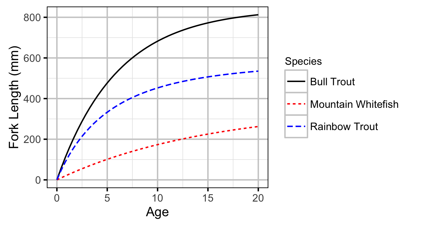
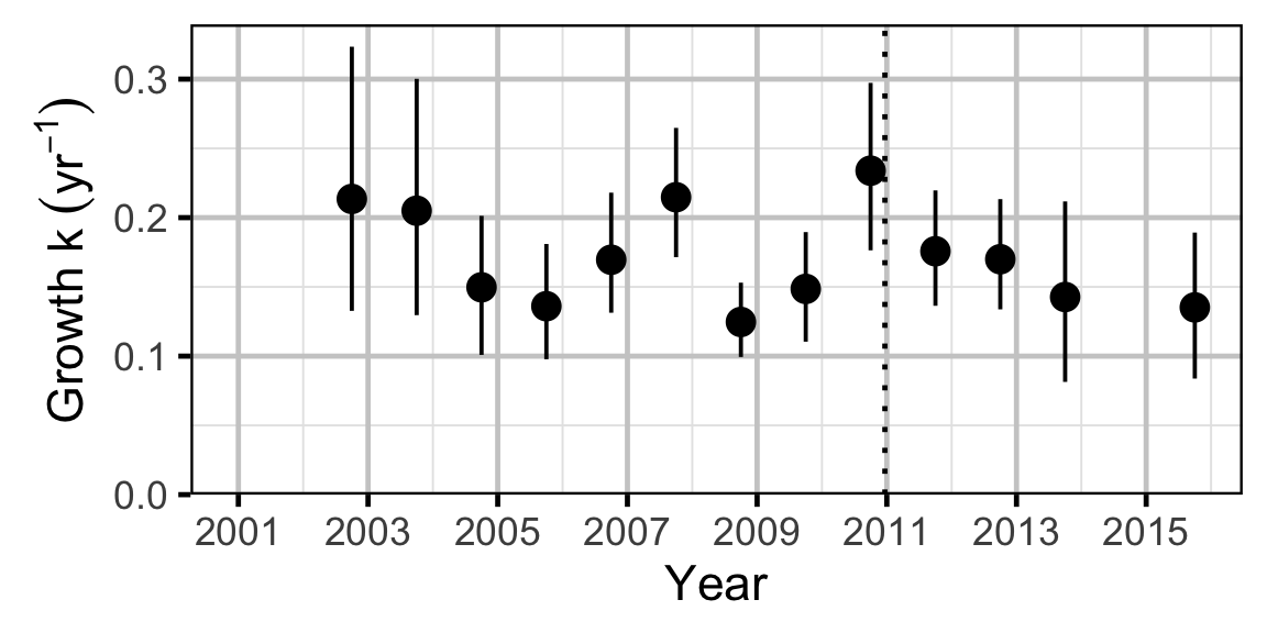
Growth - Bull Trout
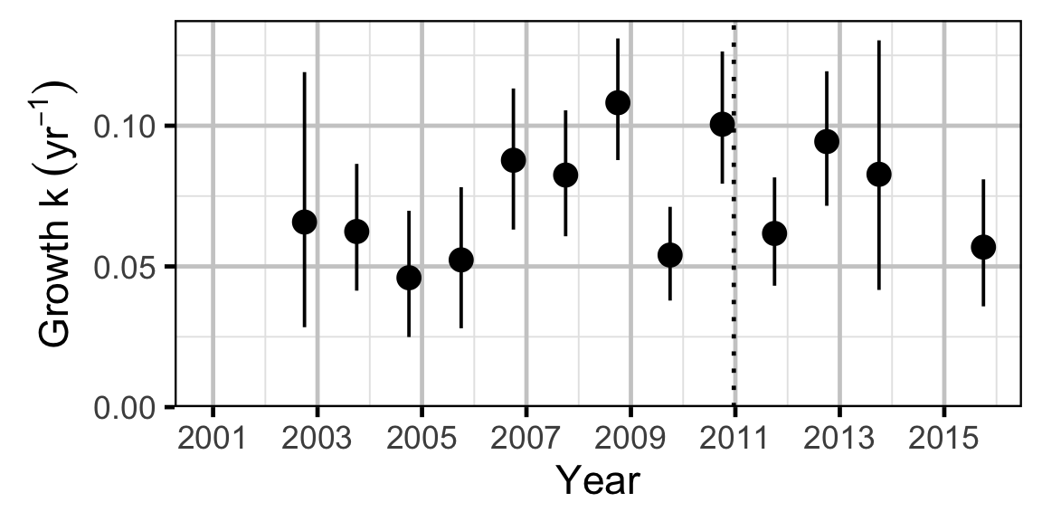
Growth - Mountain Whitefish
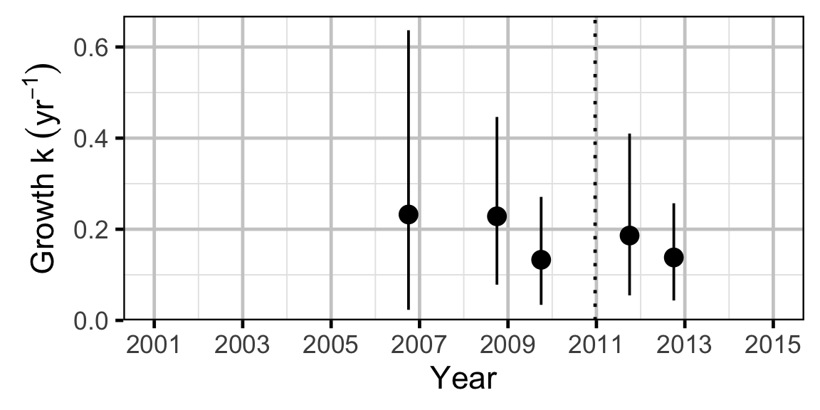
Growth - Rainbow Trout
Condition
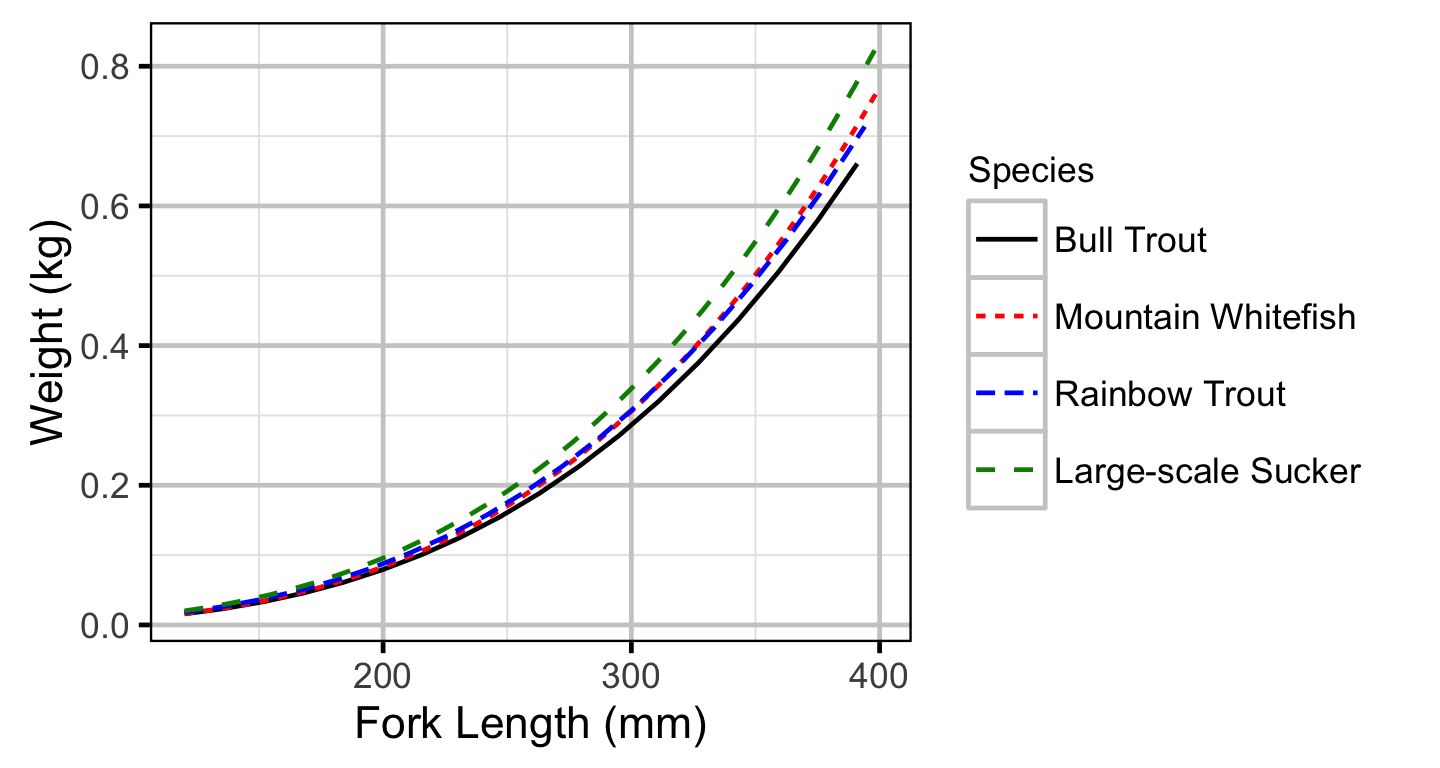
Condition - Bull Trout - Juvenile
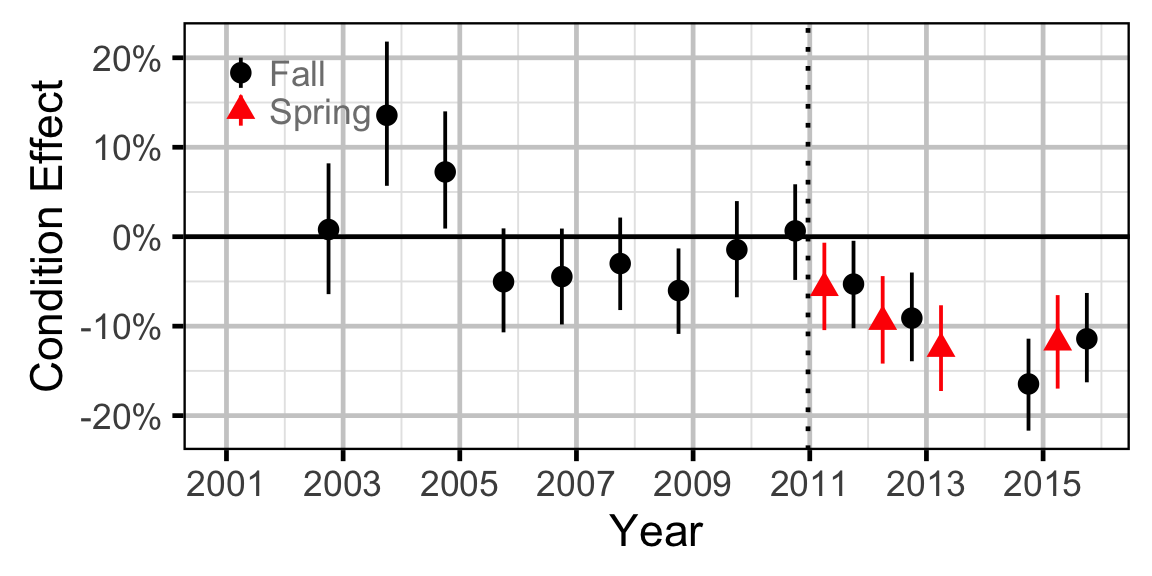
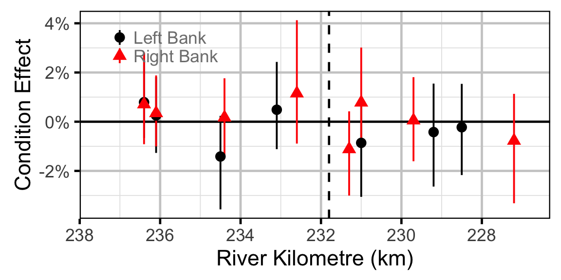
Condition - Bull Trout - Adult
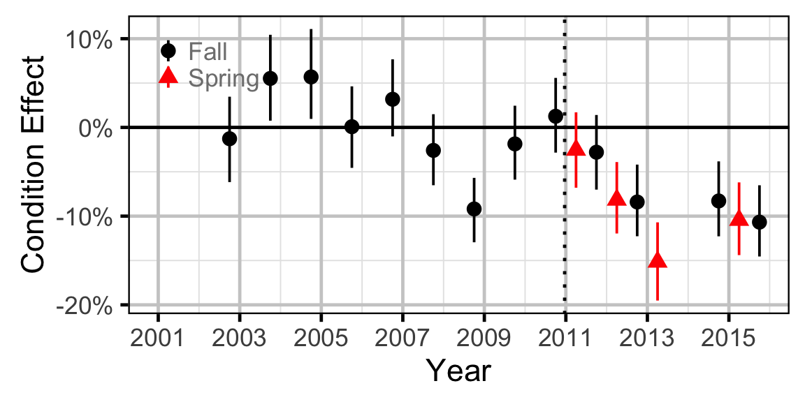

Condition - Mountain Whitefish - Juvenile
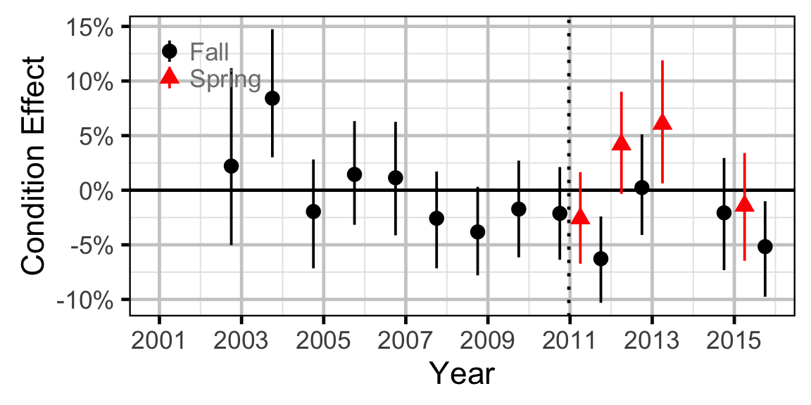
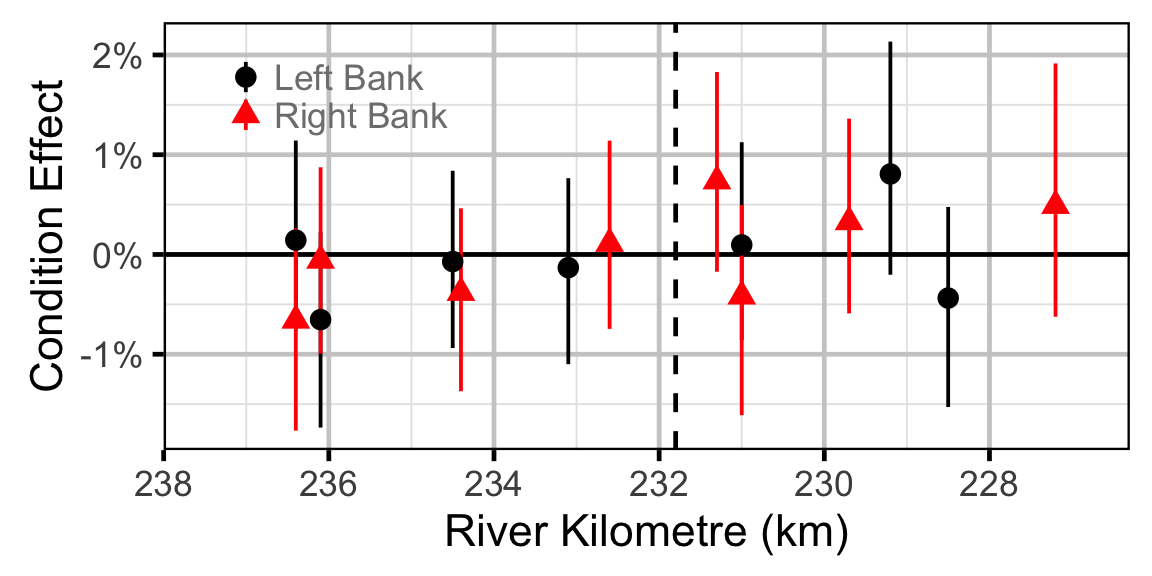
Condition - Mountain Whitefish - Adult
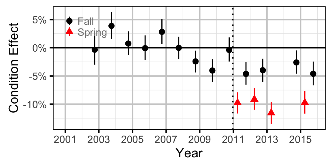

Condition - Rainbow Trout - Juvenile
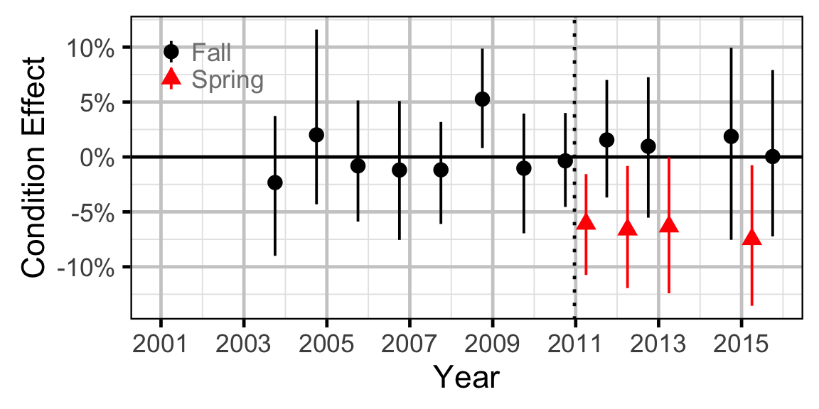
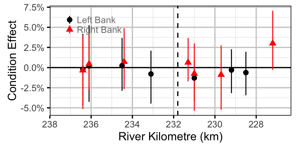
Condition - Rainbow Trout - Adult
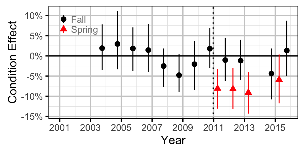

Condition - Largescale Sucker - Juvenile
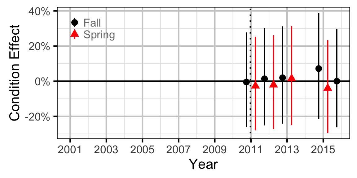
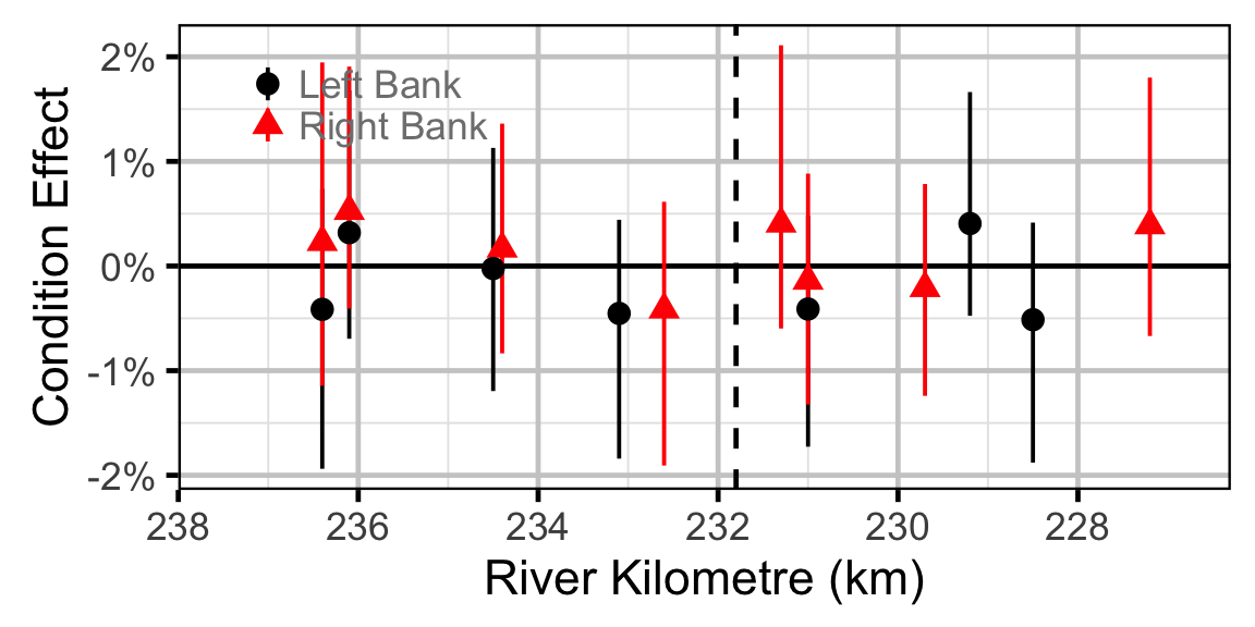
Condition - Largescale Sucker - Adult

Occupancy - Rainbow Trout
Occupancy - Burbot
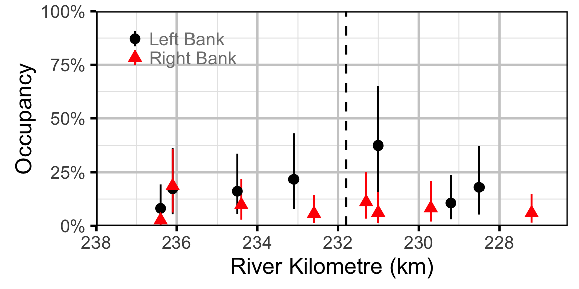
Occupancy - Lake Whitefish
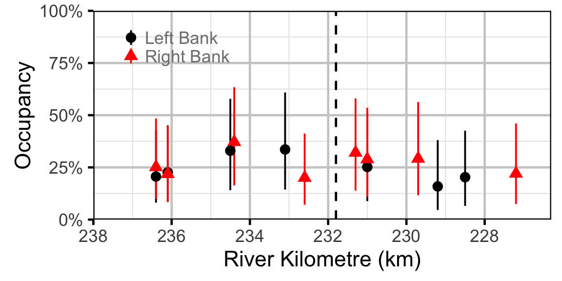
Occupancy - Northern Pikeminnow
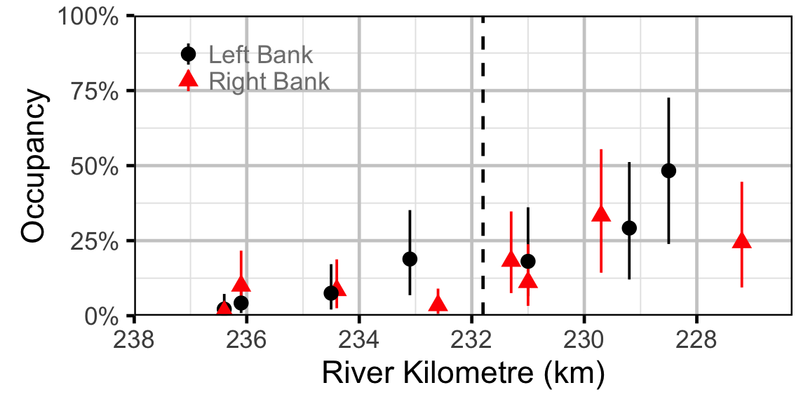
Occupancy - Redside Shiner
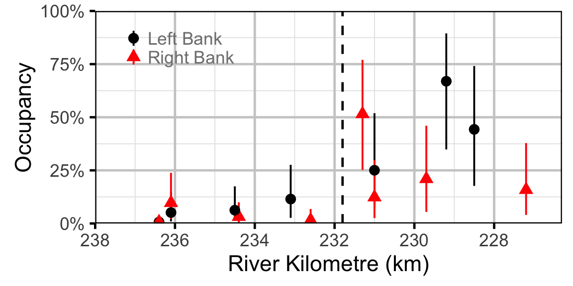
Occupancy - Sculpins
Species Richness
Count - Rainbow Trout
Count - Burbot
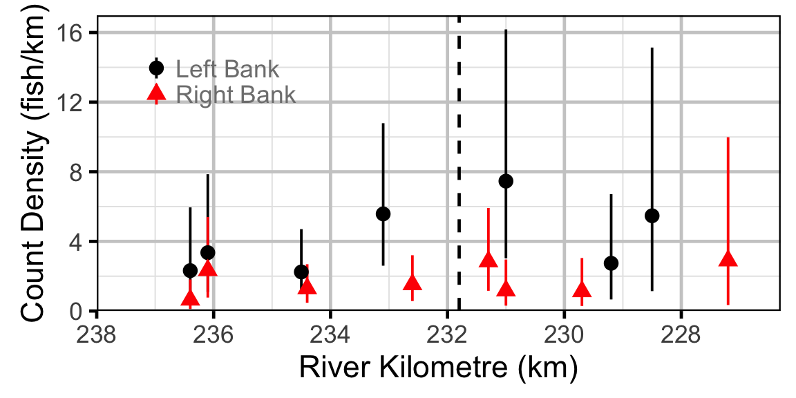
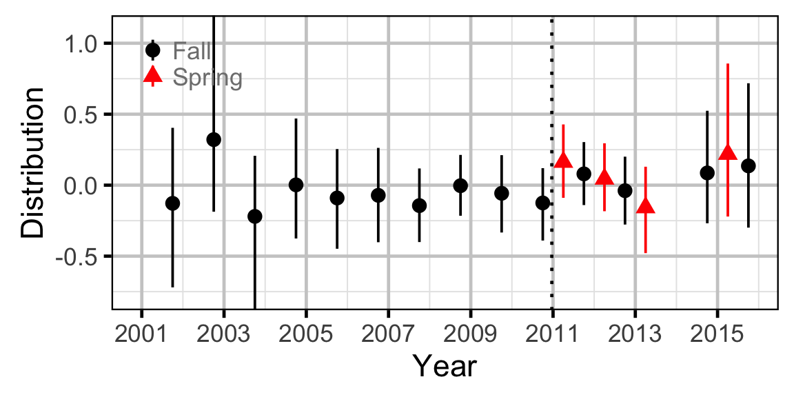
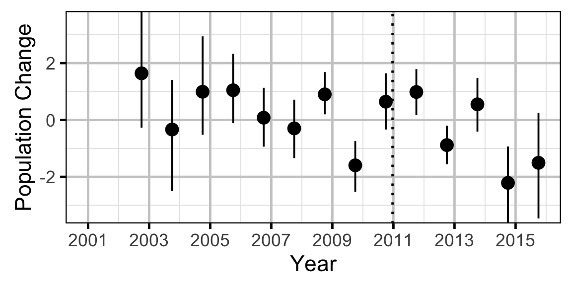
Count - Northern Pikeminnow
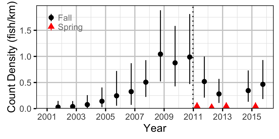
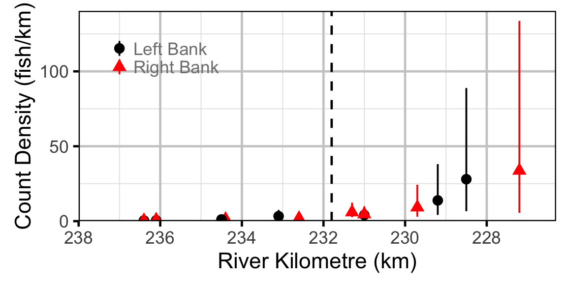
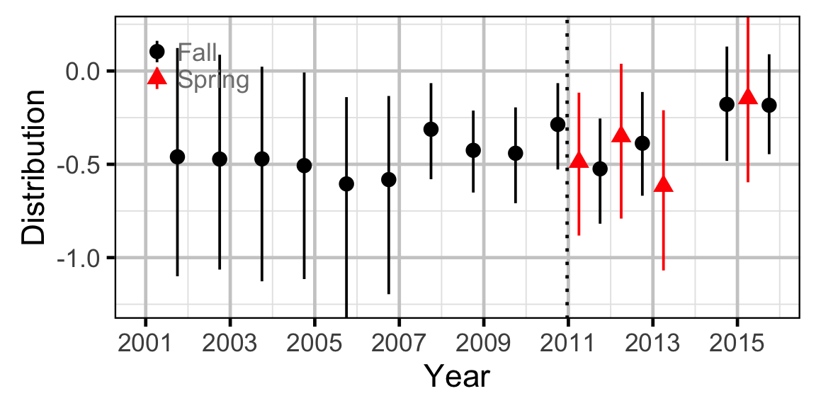
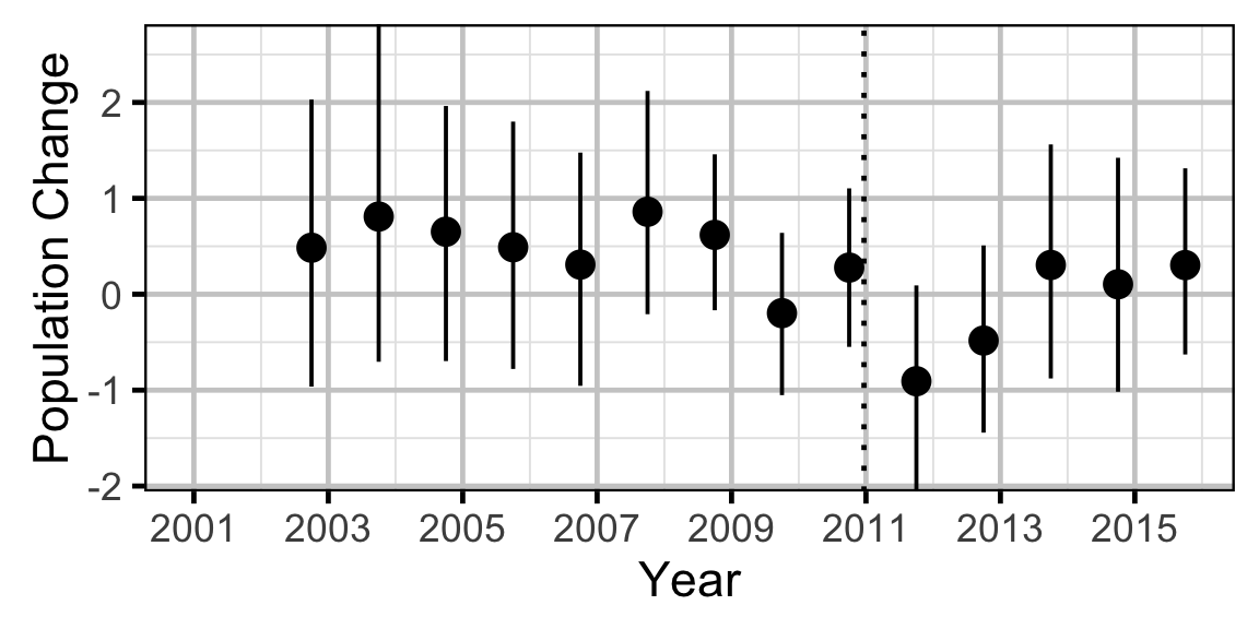
Count - Suckers
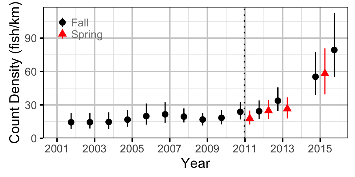
Movement - Bull Trout
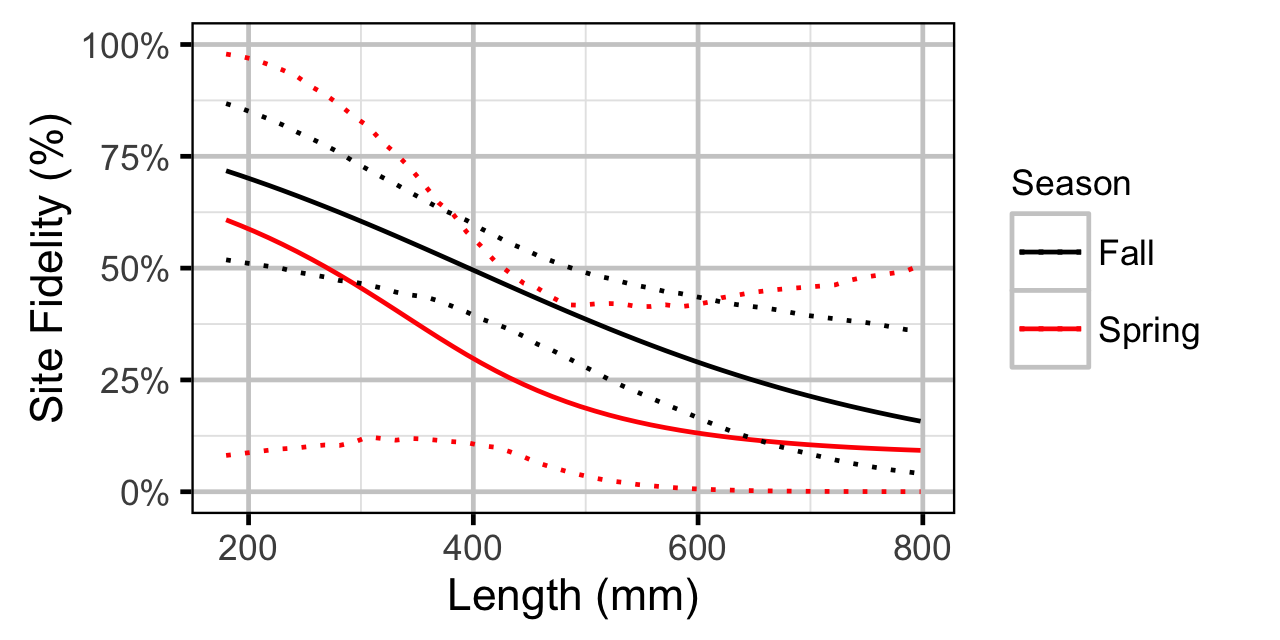
Movement - Mountain Whitefish
Movement - Rainbow Trout
Movement - Largescale Sucker
Observer Length Correction
Abundance
Abundance - Bull Trout - Adult
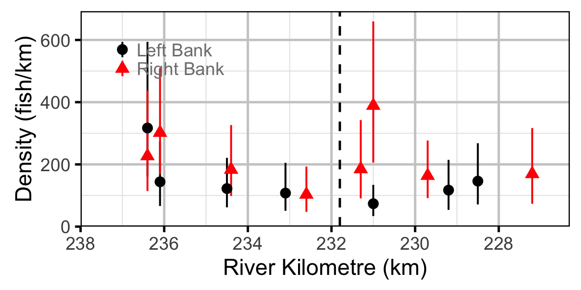
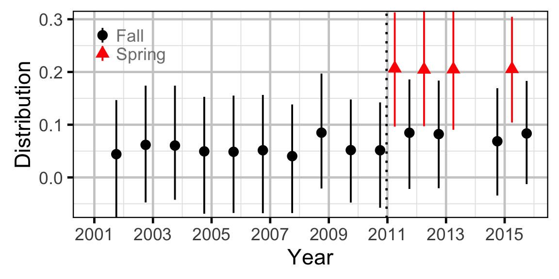
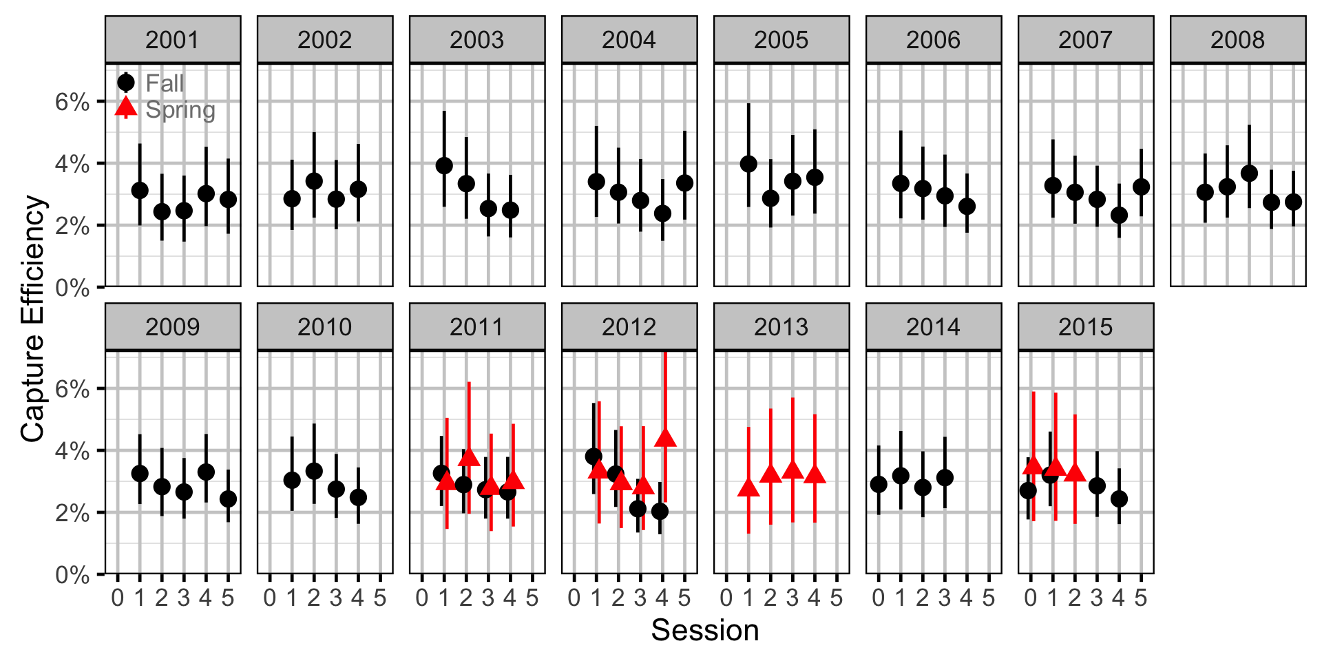
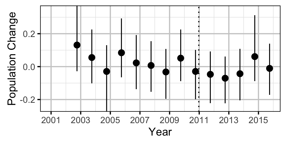
Abundance - Bull Trout - Juvenile
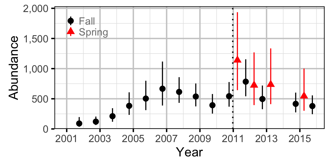
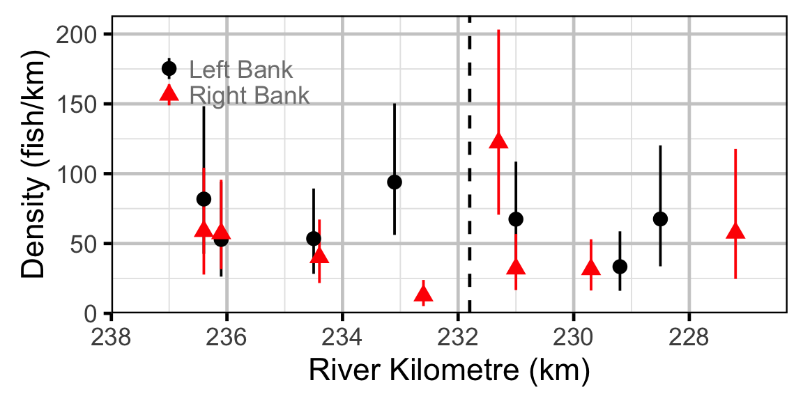
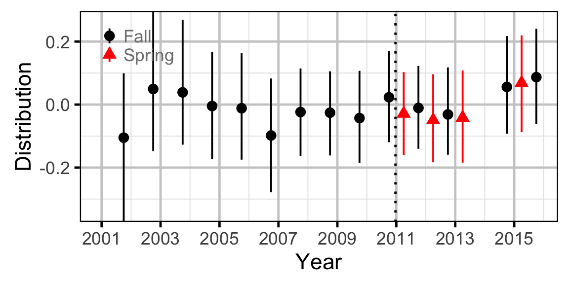
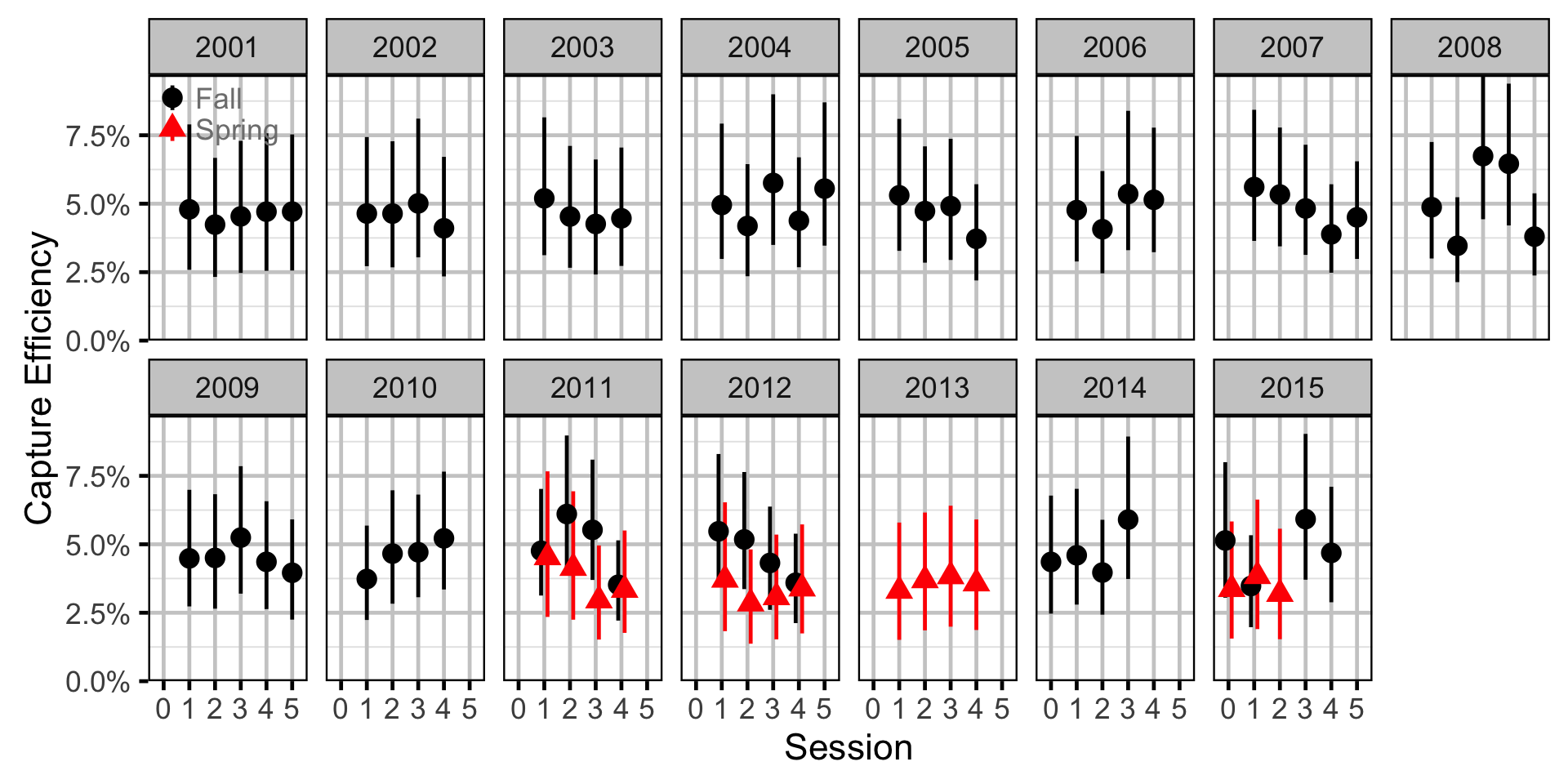
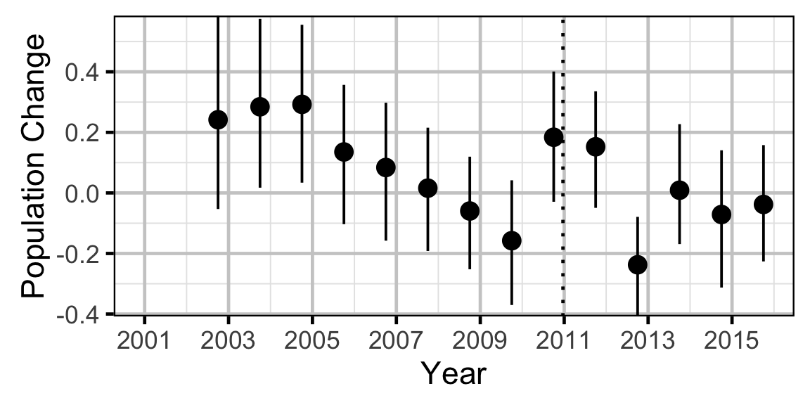
Abundance - Mountain Whitefish - Adult
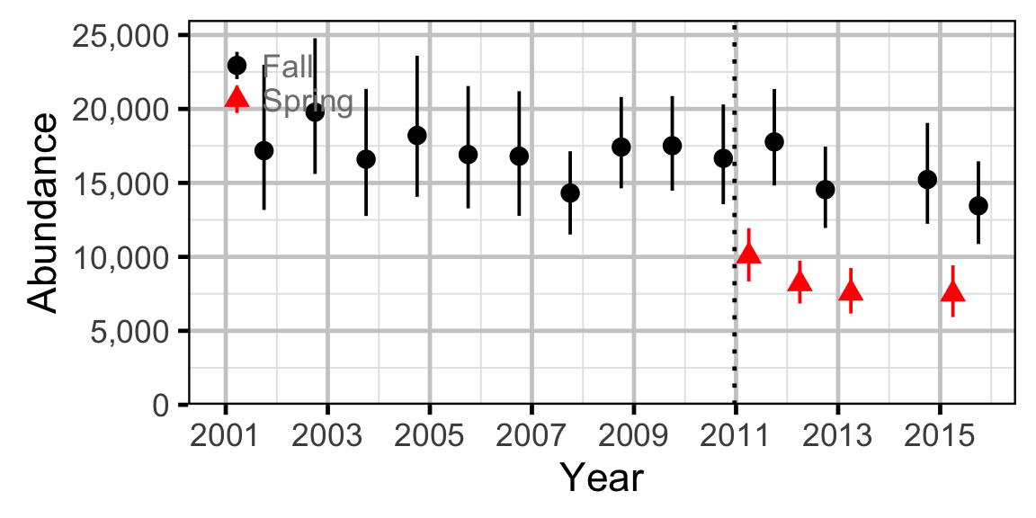
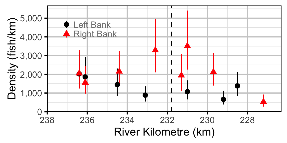
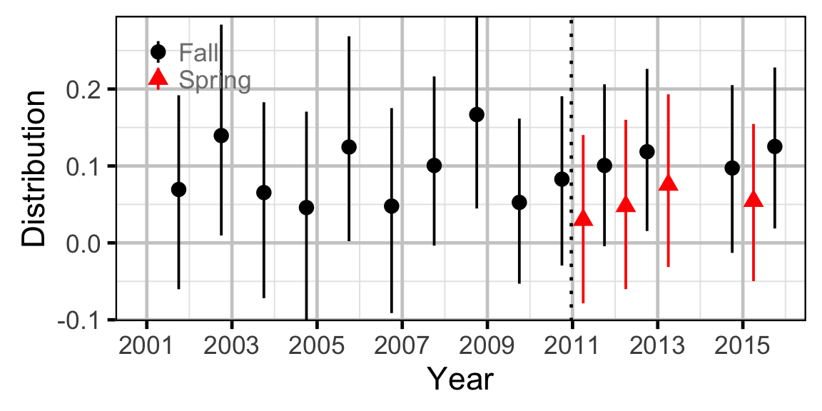
Abundance - Mountain Whitefish - Juvenile
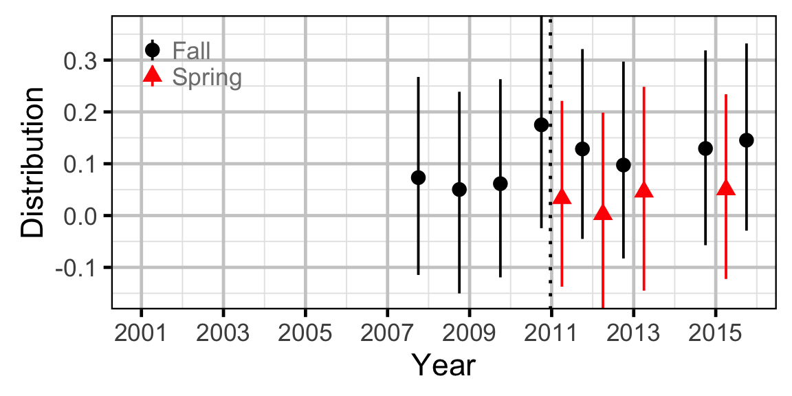
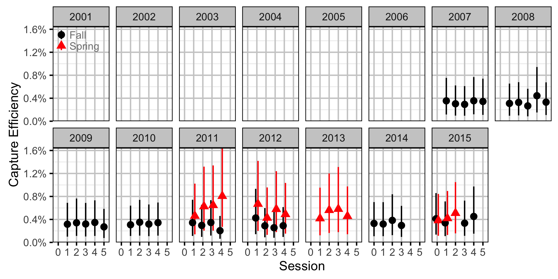
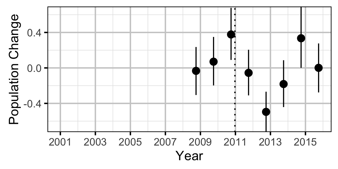
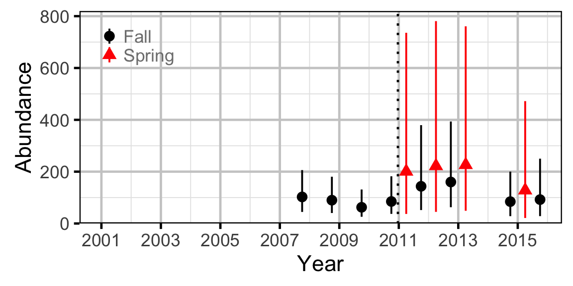
Abundance - Rainbow Trout - Adult
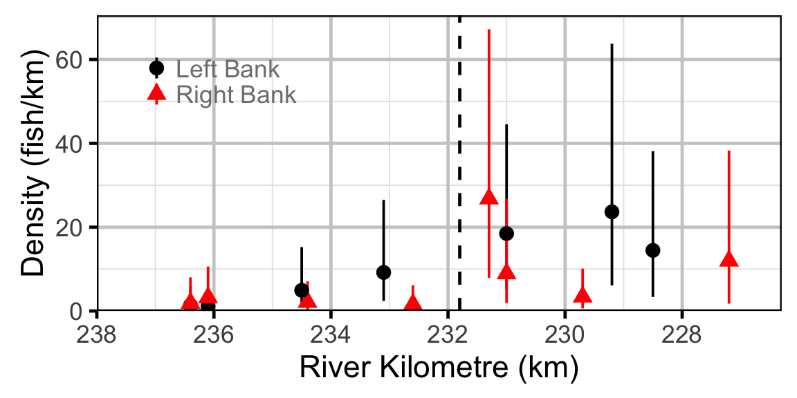
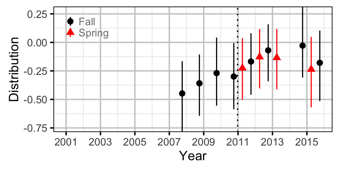
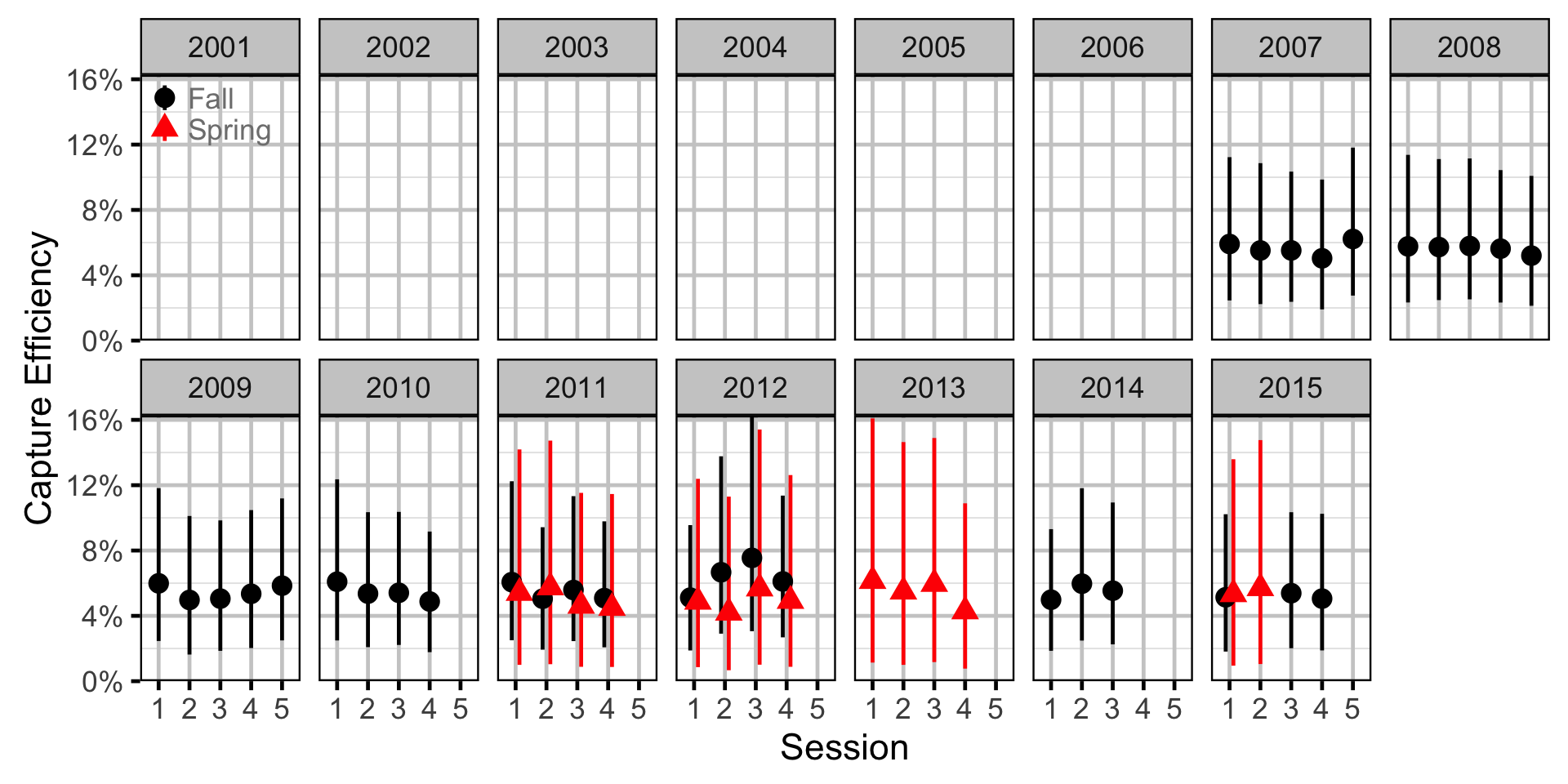
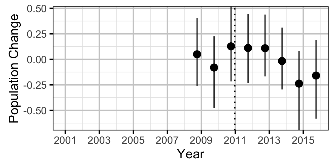
Species Diversity (Evenness)
Long-Term Trends
Short-Term Correlations
Scale Age
Significance
The following table summarises the significance levels for the management hypotheses tested in the analyses where Condition1 is the effect of the regime change on weight for big and small fish and Condition2 is the effect on big relative to small fish. The Direction column indicates whether significant changes were positive or negative where a positive change for Distribution indicates a shift towards the dam.
| Test | Species | Stage | Significance | Direction |
|---|---|---|---|---|
| Growth | Mountain Whitefish | 0.4152 | ||
| Growth | Rainbow Trout | 0.4851 | ||
| Growth | Bull Trout | 0.8823 | ||
| Condition1 | Mountain Whitefish | 0.0040 | - | |
| Condition1 | Rainbow Trout | 0.9761 | ||
| Condition1 | Bull Trout | 0.0060 | - | |
| Condition1 | Largescale Sucker | 0.1171 | ||
| Condition2 | Mountain Whitefish | 0.4152 | ||
| Condition2 | Rainbow Trout | 0.5430 | ||
| Condition2 | Bull Trout | 0.5015 | ||
| Condition2 | Largescale Sucker | 0.2044 | ||
| Abundance | Mountain Whitefish | Juvenile | 0.5579 | |
| Abundance | Mountain Whitefish | Adult | 0.4152 | |
| Abundance | Rainbow Trout | 0.0839 | ||
| Abundance | Rainbow Trout | Adult | 0.5150 | |
| Abundance | Bull Trout | Juvenile | 0.1155 | |
| Abundance | Bull Trout | Adult | 0.4951 | |
| Abundance | Sucker | 0.0417 | + | |
| Abundance | Burbot | 0.0440 | - | |
| Abundance | Northern Pikeminnow | 0.5290 | ||
| Distribution | Mountain Whitefish | Juvenile | 0.5599 | |
| Distribution | Mountain Whitefish | Adult | 0.4991 | |
| Distribution | Rainbow Trout | 0.0180 | + | |
| Distribution | Rainbow Trout | Adult | 0.0739 | |
| Distribution | Bull Trout | Juvenile | 0.4836 | |
| Distribution | Bull Trout | Adult | 0.5090 | |
| Distribution | Sucker | 0.0239 | + | |
| Distribution | Burbot | 0.6707 | ||
| Distribution | Northern Pikeminnow | 0.7446 |
Acknowledgements
The organisations and individuals whose contributions have made this analysis report possible include:
- BC Hydro
- Guy Martel
- Karen Bray
- Jason Watson
- Okanagan National Alliance
- Amy Duncan
- Michael Zimmer
- Charlotte Whitney
- Golder Associates
- David Roscoe
- Dustin Ford
- Sima Usvyatsov
- Dana Schmidt
- Larry Hildebrand
References
Abmann, C., J. Boysen-Hogrefe, and M. Pape. 2014. “Bayesian Analysis of Dynamic Factor Models: An Ex-Post Approach Towards the Rotation Problem.” Kiel Working Paper No. 1902. Kiel, Germany: Kiel Institute for the World Economy.
Bradford, Michael J, Josh Korman, and Paul S Higgins. 2005. “Using Confidence Intervals to Estimate the Response of Salmon Populations (Oncorhynchus Spp.) to Experimental Habitat Alterations.” Canadian Journal of Fisheries and Aquatic Sciences 62 (12): 2716–26. https://doi.org/10.1139/f05-179.
Fabens, A J. 1965. “Properties and Fitting of the von Bertalanffy Growth Curve.” Growth 29 (3): 265–89.
He, Ji X., James R. Bence, James E. Johnson, David F. Clapp, and Mark P. Ebener. 2008. “Modeling Variation in Mass-Length Relations and Condition Indices of Lake Trout and Chinook Salmon in Lake Huron: A Hierarchical Bayesian Approach.” Transactions of the American Fisheries Society 137 (3): 801–17. https://doi.org/10.1577/T07-012.1.
Hurlbert, S. 1984. “Pseudoreplication and the Design of Ecological Field Experiments.” Ecological Monographs 54 (2): 187–211.
Kery, Marc. 2010. Introduction to WinBUGS for Ecologists: A Bayesian Approach to Regression, ANOVA, Mixed Models and Related Analyses. Amsterdam; Boston: Elsevier. http://public.eblib.com/EBLPublic/PublicView.do?ptiID=629953.
Kery, Marc, and Michael Schaub. 2011. Bayesian Population Analysis Using WinBUGS : A Hierarchical Perspective. Boston: Academic Press. http://www.vogelwarte.ch/bpa.html.
Plummer, Martyn. 2015. “JAGS Version 4.0.1 User Manual.” http://sourceforge.net/projects/mcmc-jags/files/Manuals/4.x/.
Team, R Core. 2013. “R: A Language and Environment for Statistical Computing.” Vienna, Austria: R Foundation for Statistical Computing. http://www.R-project.org.
Thorley, J. L. 2013. “Jaggernaut: An R Package to Facilitate Bayesian Analyses Using JAGS (Just Another Gibbs Sampler).” Nelson, B.C.: Poisson Consulting Ltd. https://github.com/poissonconsulting/jaggernaut.
von Bertalanffy, L. 1938. “A Quantitative Theory of Organic Growth (Inquiries on Growth Laws Ii).” Human Biology 10: 181–213.
Zuur, A F, I D Tuck, and N Bailey. 2003. “Dynamic Factor Analysis to Estimate Common Trends in Fisheries Time Series.” Canadian Journal of Fisheries and Aquatic Sciences 60 (5): 542–52. https://doi.org/10.1139/f03-030.