Mackenzie Wood Bison Population Dynamics Analysis 2015
The suggested citation for this analytic report is:
Thorley, J.L. and Boulanger, J. (2015) Mackenzie Wood Bison Population Dynamics Analysis 2015. A Poisson Consulting Analysis Report. URL: https://www.poissonconsulting.ca/f/164478860.
Background
The Mackenzie Wood Bison (Bison bison athabascae) herd abundance has been estimated in four years since 1999 while herd composition data has been collected in all but three years. The herd composition data is collected in July while the abundance estimates are for March.
The primary questions this analysis attempts to answer are:
What is the survival of calves, yearlings and adult in the Mackenzie herd?
Is survival of calves in the Mackenzie herd driven by climatic conditions?
Methods
Data Preparation
The data were provided by Aurora Consulting, the University of Alberta and the Government of the Northwest Territories.
In 2013 the herd experienced high mortality due to an anthrax outbreak. Consequently, the 2013 and 2014 data were excluded.
Statistical Analysis
Hierarchical Bayesian models were fitted to the data using R version 3.2.0 (Team 2013) and JAGS 3.4.0 (Plummer 2012) which interfaced with each other via jaggernaut 2.2.10 (Thorley 2013). For additional information on hierarchical Bayesian modelling in the BUGS language, of which JAGS uses a dialect, the reader is referred to Kery and Schaub (2011, 41–44).
Unless specified, the models assumed vague (low information) prior distributions (Kery and Schaub 2011, 36). The posterior distributions were estimated from a minimum of 1,000 Markov Chain Monte Carlo (MCMC) samples thinned from the second halves of three chains (Kery and Schaub 2011, 38–40). Model convergence was confirmed by ensuring that Rhat (Kery and Schaub 2011, 40) was less than 1.1 for each of the parameters in the model (Kery and Schaub 2011, 61). Model adequacy was confirmed by examination of residual plots.
The posterior distributions of the fixed (Kery and Schaub 2011, 75) parameters are summarised in terms of a point estimate (mean), lower and upper 95% credible limits (2.5th and 97.5th percentiles), the standard deviation (SD), percent relative error (half the 95% credible interval as a percent of the point estimate) and significance (Kery and Schaub 2011, 37, 42).
Variable selection was achieved by dropping insignificant (Kery and Schaub 2011, 37, 42) fixed (Kery and Schaub 2011, 77–82) variables and uninformative random variables. A fixed variables was considered to be insignificant if its significance was \(\geq\) 0.05 while a random variable was considered to be uninformative if its percent relative error was \(\geq\) 80%.
The results are displayed graphically by plotting the modeled relationships between particular variables and the response with 95% credible intervals (CRIs) with the remaining variables held constant. In general, continuous and discrete fixed variables are held constant at their mean and first level values respectively while random variables are held constant at their typical values (expected values of the underlying hyperdistributions) (Kery and Schaub 2011, 77–82). Where informative the influence of particular variables is expressed in terms of the effect size (i.e., percent change in the response variable) with 95% CRIs (Bradford, Korman, and Higgins 2005).
Model Description
The following model description observes several conventions.
The survival between life stages was estimated using a hierarchical Bayesian population dynamic state-space model (Kery and Schaub 2011). Key assumptions of the population dynamic model include:
- A 50:50 sex ratio.
- Constant probability of a female adult calfing.
- Annually varying calf survival.
- Calf survival is able to vary with the Pacific Decadal Oscillation Index.
- Constant and identical yearling and adult survival.
- Clustering of cows with and without calves.
- Each year runs from May 15 to May 15.
- Survival does not vary seasonally.
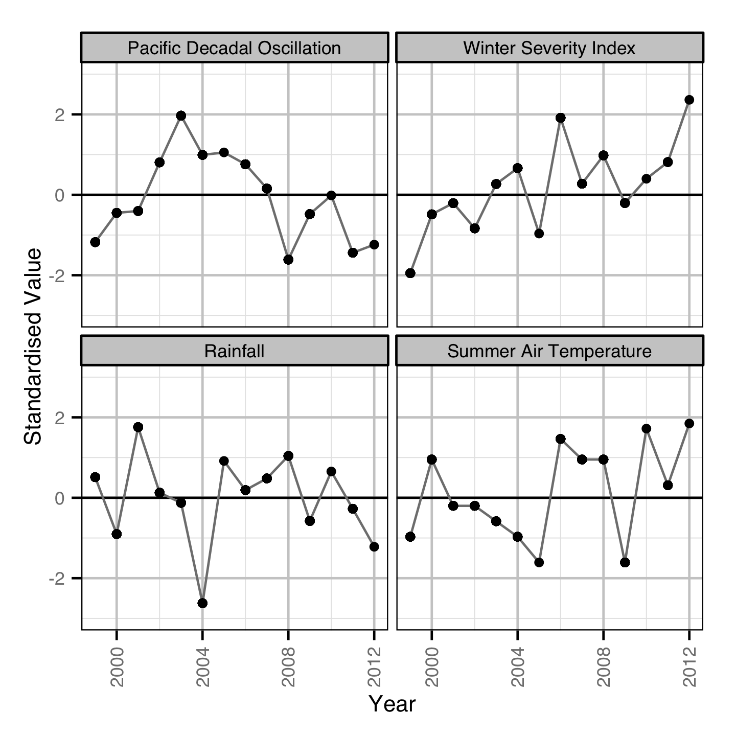
In addition the effect of various environmental variables on calf survival was tested by adding a standardised covariate to the population dynamic model.
Model Code
The JAGS model code, which uses a series of naming conventions, is presented below.
Population Dynamic
| Variable/Parameter | Description |
|---|---|
bAdults[i] |
Number of adults at the start of the i\(^{th}\) year |
bAdults1 |
Number of adults at the start of the first year |
bCalves[i] |
Number of calves at the start of the i\(^{th}\) year |
Bison[i] |
The i\(^{th}\) herd size estimate |
bProductivity |
Probability of a female adult calving |
bSurvivalAdult |
Adult and yearling survival |
bSurvivalCalf |
Calf survival |
bYearlings[i] |
Number of yearlings at the start of the i\(^{th}\) year |
bYearlings1 |
Number of yearlings at the start of the first year |
Calves[i] |
Number of calves in the i\(^{th}\) composition observation |
Cows[i] |
Number of cows in the i\(^{th}\) composition observation |
Dayte[i] |
Day of the year of the i\(^{th}\) composition observation |
eCorrection |
Survival correction for the timing of the herd size estimates |
eProportionCalves[i] |
Expected proportion of cows with a calf in the i\(^{th}\) composition observation |
eProportionCowsYearlings[i] |
Expected proportion of cows and yearlings that are cows in the i\(^{th}\) composition observation |
eSurvivalCalfYear[i] |
Calf survival from the i\(^{th}\) to i+1\(^{th}\) year |
sDispersionCalves |
SD of the extra-binomial variation in cow with calf clustering |
sSurvivalCalfYear |
SD of the effect of year on bSurvivalCalf |
YearBison[i] |
The year of the i\(^{th}\) herd size estimate |
YearlingsCows[i] |
Number of yearlings and cows in the i\(^{th}\) composition observation |
Population Dynamic - Model1
model{

  bProductivity ~ dunif(0, 1)
  bSurvivalAdult ~ dunif(0, 1)
  bSurvivalCalf ~ dunif(0, 1)

  sSurvivalCalfYear ~ dunif(0, 2)
  for(i in 1:nYear){
    bSurvivalCalfYear[i] ~ dnorm(0, sSurvivalCalfYear^-2)
    logit(eSurvivalCalfYear[i]) <- logit(bSurvivalCalf) + bSurvivalCalfYear[i]
  }

  bYearlings1 ~ dunif(0, 500)
  bAdults1 ~ dunif(0, 4000)

  bCalves[1] <- bAdults1 / 2 * bProductivity
  bYearlings[1] <- bYearlings1
  bAdults[1] <- bAdults1

  for(i in 2:nYear){
    bCalves[i] <- bAdults[i-1] / 2 * bSurvivalAdult * bProductivity
    bYearlings[i] <- bCalves[i-1] * eSurvivalCalfYear[i-1]
    bAdults[i] <- (bYearlings[i-1] + bAdults[i-1]) * bSurvivalAdult
  }

  eCorrection <- 308/365
  for(i in 1:length(YearBison)) {
    eCalves[i] <- bCalves[YearBison[i]] * eSurvivalCalfYear[YearBison[i]]^eCorrection
    eYearlings[i] <- bYearlings[YearBison[i]] * bSurvivalAdult^eCorrection
    eAdults[i] <- bAdults[YearBison[i]] * bSurvivalAdult^eCorrection

    eBison[i] <- eCalves[i] + eYearlings[i] + eAdults[i]
    Bison[i] ~ dnorm(eBison[i], 250^-2)
  }

  sDispersionCalves ~ dunif(0, 2)
  for(i in 1:length(Year)) {
    eCorComp[i] <- ((Dayte[i] - 135) / 365)
    eCalvesComp[i] <- bCalves[Year[i]] * eSurvivalCalfYear[Year[i]]^eCorComp[i]
    eYearlingsComp[i] <- bYearlings[Year[i]] * bSurvivalAdult^eCorComp[i]
    eAdultsComp[i] <- bAdults[Year[i]] * bSurvivalAdult^eCorComp[i]

    eCowsComp[i] <- eAdultsComp[i] / 2

    eDispersionCalves[i] ~ dnorm(0, sDispersionCalves^-2)
    logit(eProportionCalves[i]) <- logit(eCalvesComp[i] / eCowsComp[i]) + eDispersionCalves[i]
    eProportionCowsYearlings[i] <- eCowsComp[i] / (eYearlingsComp[i] + eCowsComp[i])

    Calves[i] ~ dbin(eProportionCalves[i], Cows[i])
    Cows[i] ~ dbin(eProportionCowsYearlings[i], YearlingsCows[i])
  }
}
Environmental
| Variable/Parameter | Description |
|---|---|
bSurvivalCalfEnv |
Effect of the environmental variable on bSurvivalCalf |
Environmental - Model1
model{

  bProductivity ~ dunif(0, 1)
  bSurvivalAdult ~ dunif(0, 1)
  bSurvivalCalf ~ dunif(0, 1)

  bSurvivalCalfEnv ~ dnorm(0, 2^-2)
  sSurvivalCalfYear ~ dunif(0, 2)
  for(i in 1:nYear){
    bSurvivalCalfYear[i] ~ dnorm(0, sSurvivalCalfYear^-2)
    logit(eSurvivalCalfYear[i]) <- logit(bSurvivalCalf) + bSurvivalCalfEnv * Env[i] + bSurvivalCalfYear[i]
  }

  bYearlings1 ~ dunif(0, 500)
  bAdults1 ~ dunif(0, 4000)

  bCalves[1] <- bAdults1 / 2 * bProductivity
  bYearlings[1] <- bYearlings1
  bAdults[1] <- bAdults1

  for(i in 2:nYear){
    bCalves[i] <- bAdults[i-1] / 2 * bSurvivalAdult * bProductivity
    bYearlings[i] <- bCalves[i-1] * eSurvivalCalfYear[i-1]
    bAdults[i] <- (bYearlings[i-1] + bAdults[i-1]) * bSurvivalAdult
  }

  eCorrection <- 308/365
  for(i in 1:length(YearBison)) {
    eCalves[i] <- bCalves[YearBison[i]] * eSurvivalCalfYear[YearBison[i]]^eCorrection
    eYearlings[i] <- bYearlings[YearBison[i]] * bSurvivalAdult^eCorrection
    eAdults[i] <- bAdults[YearBison[i]] * bSurvivalAdult^eCorrection

    eBison[i] <- eCalves[i] + eYearlings[i] + eAdults[i]
    Bison[i] ~ dnorm(eBison[i], 250^-2)
  }

  sDispersionCalves ~ dunif(0, 2)
  for(i in 1:length(Year)) {
    eCorComp[i] <- ((Dayte[i] - 135) / 365)
    eCalvesComp[i] <- bCalves[Year[i]] * eSurvivalCalfYear[Year[i]]^eCorComp[i]
    eYearlingsComp[i] <- bYearlings[Year[i]] * bSurvivalAdult^eCorComp[i]
    eAdultsComp[i] <- bAdults[Year[i]] * bSurvivalAdult^eCorComp[i]

    eCowsComp[i] <- eAdultsComp[i] / 2

    eDispersionCalves[i] ~ dnorm(0, sDispersionCalves^-2)
    logit(eProportionCalves[i]) <- logit(eCalvesComp[i] / eCowsComp[i]) + eDispersionCalves[i]
    eProportionCowsYearlings[i] <- eCowsComp[i] / (eYearlingsComp[i] + eCowsComp[i])

    Calves[i] ~ dbin(eProportionCalves[i], Cows[i])
    Cows[i] ~ dbin(eProportionCowsYearlings[i], YearlingsCows[i])
  }
}
Results
Model Parameters
The posterior distributions for the fixed (Kery and Schaub 2011 p. 75) parameters in each model are summarised below.
Population Dynamic
| Parameter | Estimate | Lower | Upper | SD | Error | Significance |
|---|---|---|---|---|---|---|
| bAdults1 | 1780.00000 | 1273.00000 | 2303.00000 | 259.00000 | 29 | 0.001 |
| bProductivity | 0.45970 | 0.40530 | 0.51670 | 0.02960 | 12 | 0.001 |
| bSurvivalAdult | 0.88991 | 0.85823 | 0.92207 | 0.01622 | 4 | 0.001 |
| bSurvivalCalf | 0.44130 | 0.32300 | 0.60060 | 0.07020 | 31 | 0.001 |
| bYearlings1 | 279.70000 | 185.10000 | 381.60000 | 48.40000 | 35 | 0.001 |
| sDispersionCalves | 0.74820 | 0.60320 | 0.91880 | 0.08010 | 21 | 0.001 |
| sSurvivalCalfYear | 0.66580 | 0.33460 | 1.23600 | 0.23260 | 68 | 0.001 |
| Convergence | Iterations |
|---|---|
| 1.01 | 1e+05 |
Environmental - Pacific Decadal Oscillation
| Parameter | Estimate | Lower | Upper | SD | Error | Significance |
|---|---|---|---|---|---|---|
| bAdults1 | 1763.0000 | 1283.00000 | 2290.00000 | 261.00000 | 29 | 0.0010 |
| bProductivity | 0.4550 | 0.40150 | 0.51470 | 0.02940 | 12 | 0.0010 |
| bSurvivalAdult | 0.8910 | 0.86025 | 0.92222 | 0.01589 | 3 | 0.0010 |
| bSurvivalCalf | 0.4459 | 0.33070 | 0.57910 | 0.06430 | 28 | 0.0010 |
| bSurvivalCalfEnv | -0.3077 | -0.73910 | 0.13260 | 0.22140 | 140 | 0.1378 |
| bYearlings1 | 277.6000 | 191.50000 | 379.90000 | 47.70000 | 34 | 0.0010 |
| sDispersionCalves | 0.7528 | 0.60290 | 0.93010 | 0.08200 | 22 | 0.0010 |
| sSurvivalCalfYear | 0.6090 | 0.24400 | 1.28700 | 0.25900 | 86 | 0.0010 |
| Convergence | Iterations |
|---|---|
| 1.01 | 1e+05 |
Environmental - Winter Severity Index
| Parameter | Estimate | Lower | Upper | SD | Error | Significance |
|---|---|---|---|---|---|---|
| bAdults1 | 1768.00000 | 1293.00000 | 2306.00000 | 260.00000 | 29 | 0.0010 |
| bProductivity | 0.45660 | 0.40040 | 0.51560 | 0.02950 | 13 | 0.0010 |
| bSurvivalAdult | 0.88925 | 0.85634 | 0.92127 | 0.01612 | 4 | 0.0010 |
| bSurvivalCalf | 0.44660 | 0.31550 | 0.59530 | 0.07000 | 31 | 0.0010 |
| bSurvivalCalfEnv | 0.17980 | -0.28890 | 0.67070 | 0.24050 | 270 | 0.3893 |
| bYearlings1 | 276.70000 | 189.90000 | 374.20000 | 48.80000 | 33 | 0.0010 |
| sDispersionCalves | 0.74890 | 0.59600 | 0.91360 | 0.08140 | 21 | 0.0010 |
| sSurvivalCalfYear | 0.69000 | 0.32500 | 1.34500 | 0.25000 | 74 | 0.0010 |
| Convergence | Iterations |
|---|---|
| 1.01 | 1e+05 |
Environmental - Rainfall
| Parameter | Estimate | Lower | Upper | SD | Error | Significance |
|---|---|---|---|---|---|---|
| bAdults1 | 1785.50000 | 1294.10000 | 2285.60000 | 256.10000 | 28 | 0.0010 |
| bProductivity | 0.46020 | 0.40370 | 0.52020 | 0.02970 | 13 | 0.0010 |
| bSurvivalAdult | 0.88934 | 0.85726 | 0.92169 | 0.01665 | 4 | 0.0010 |
| bSurvivalCalf | 0.44340 | 0.30310 | 0.61400 | 0.07660 | 35 | 0.0010 |
| bSurvivalCalfEnv | -0.00900 | -0.60000 | 0.56900 | 0.29700 | 6700 | 0.9781 |
| bYearlings1 | 281.70000 | 189.90000 | 387.00000 | 50.00000 | 35 | 0.0010 |
| sDispersionCalves | 0.74970 | 0.59400 | 0.92190 | 0.07990 | 22 | 0.0010 |
| sSurvivalCalfYear | 0.71800 | 0.35500 | 1.37300 | 0.26000 | 71 | 0.0010 |
| Convergence | Iterations |
|---|---|
| 1.01 | 1e+05 |
Environmental - Summer Air Temperature
| Parameter | Estimate | Lower | Upper | SD | Error | Significance |
|---|---|---|---|---|---|---|
| bAdults1 | 1771.20000 | 1301.40000 | 2269.50000 | 252.70000 | 27 | 0.0010 |
| bProductivity | 0.45900 | 0.40270 | 0.51810 | 0.02970 | 13 | 0.0010 |
| bSurvivalAdult | 0.89212 | 0.86129 | 0.92205 | 0.01558 | 3 | 0.0010 |
| bSurvivalCalf | 0.42610 | 0.30690 | 0.57820 | 0.06710 | 32 | 0.0010 |
| bSurvivalCalfEnv | 0.31410 | -0.12770 | 0.75160 | 0.21490 | 140 | 0.1378 |
| bYearlings1 | 277.30000 | 197.10000 | 377.40000 | 46.40000 | 33 | 0.0010 |
| sDispersionCalves | 0.74130 | 0.59450 | 0.91120 | 0.08130 | 21 | 0.0010 |
| sSurvivalCalfYear | 0.60890 | 0.28370 | 1.12560 | 0.22700 | 69 | 0.0010 |
| Convergence | Iterations |
|---|---|
| 1.01 | 1e+05 |
Figures
Population Dynamic
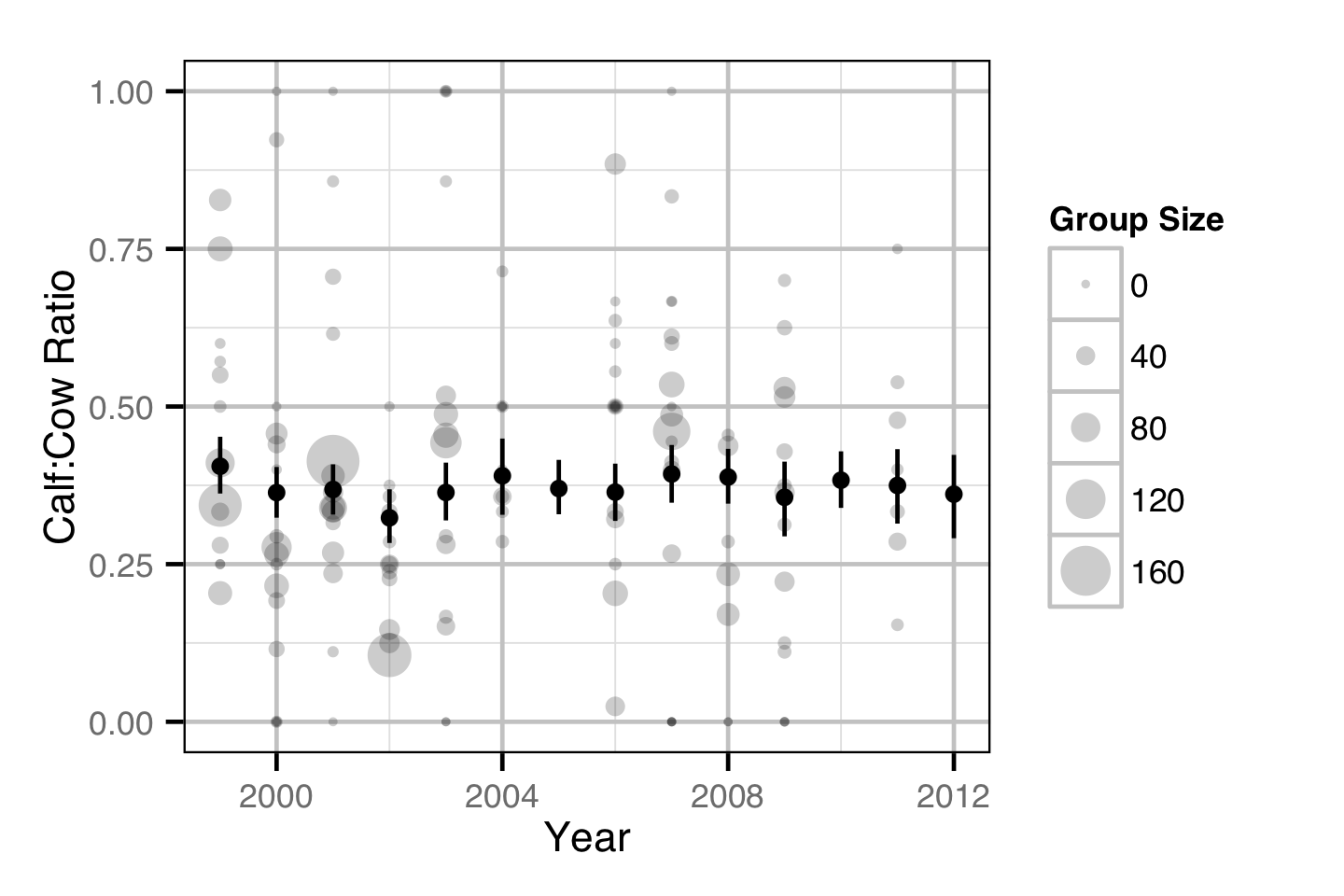
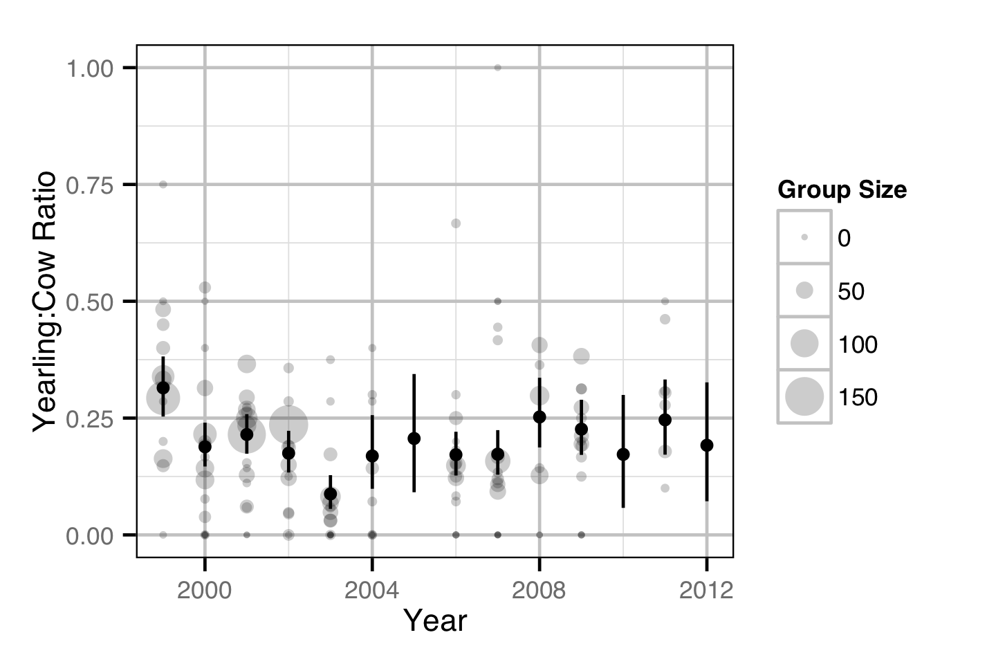
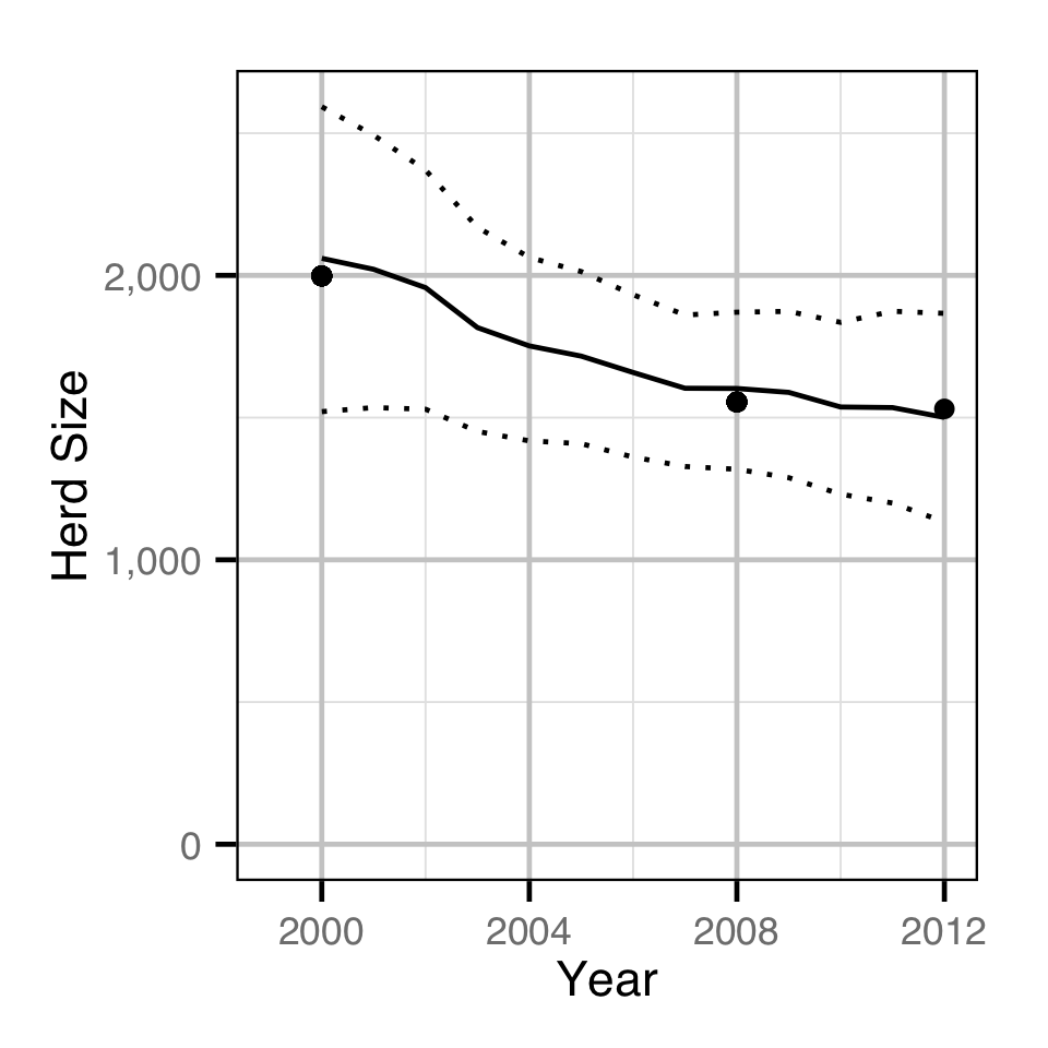
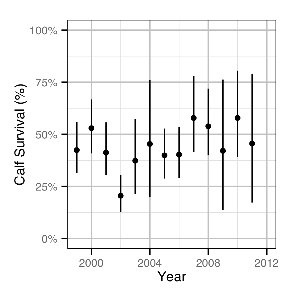
Environmental
Acknowledgements
The organisations and individuals whose contributions have made this analysis report possible include:
- Aurora Consulting
- Kim Poole
- University of Alberta
- Craig Demars
- Government of the Northwest Territorie
- Terry Armstrong
- Poisson Consulting
- Robyn Irvine
References
Bradford, Michael J, Josh Korman, and Paul S Higgins. 2005. “Using Confidence Intervals to Estimate the Response of Salmon Populations (Oncorhynchus Spp.) to Experimental Habitat Alterations.” Canadian Journal of Fisheries and Aquatic Sciences 62 (12): 2716–26. https://doi.org/10.1139/f05-179.
Kery, Marc, and Michael Schaub. 2011. Bayesian Population Analysis Using WinBUGS : A Hierarchical Perspective. Boston: Academic Press. http://www.vogelwarte.ch/bpa.html.
Plummer, Martyn. 2012. “JAGS Version 3.3.0 User Manual.” http://sourceforge.net/projects/mcmc-jags/files/Manuals/3.x/.
Team, R Core. 2013. “R: A Language and Environment for Statistical Computing.” Vienna, Austria: R Foundation for Statistical Computing. http://www.R-project.org.
Thorley, J. L. 2013. “Jaggernaut: An R Package to Facilitate Bayesian Analyses Using JAGS (Just Another Gibbs Sampler).” Nelson, B.C.: Poisson Consulting Ltd. https://github.com/poissonconsulting/jaggernaut.