Lower Duncan River Rainbow Trout Spawning Analysis 2017
The suggested citation for this analytic report is:
Thorley, J.L. & Dalgarno, S.I.J. (2018) Lower Duncan River Rainbow Trout Spawning Analysis 2017. A Poisson Consulting Analysis Report. URL: https://www.poissonconsulting.ca/f/897442882.
Background
The Lardeau River (LAR) flows 45 km from Trout Lake to join the Lower Duncan River approximately 1 km downstream of Duncan Dam (DDM). The Duncan River downstream of the Lardeau River (DRL) then extends a further 11 km downstream to Kootenay Lake. The study area for this analysis is the Duncan Above Lardeau station (DAL), located between the end of the DDM discharge channel and the confluence with the Lardeau River.
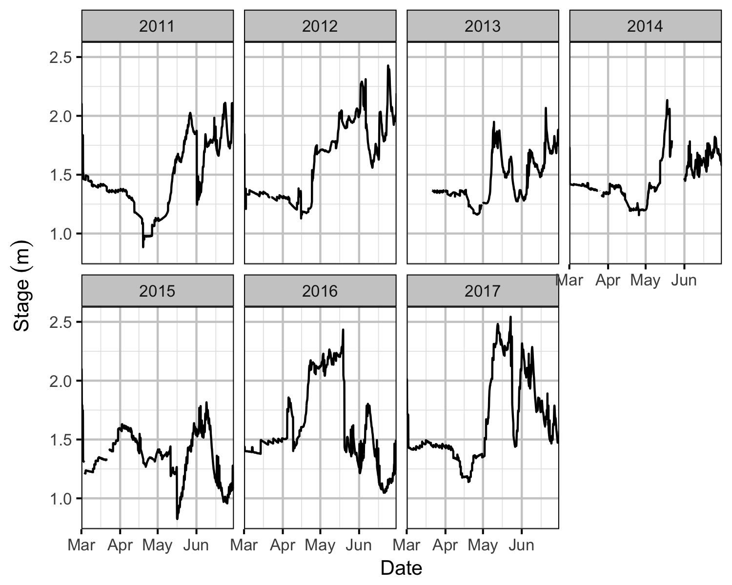
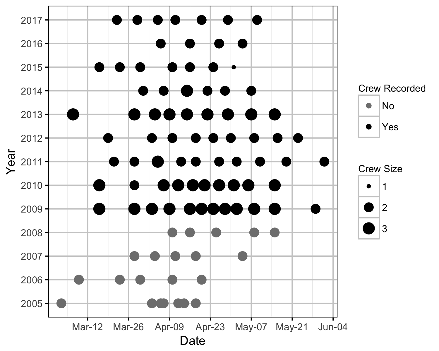
Rainbow Trout spawning below DDM has been monitored since 2005 by periodic redd surveys. Since 2011, the river stage at DAL has been recorded.
The main objectives of the current analyses were to:
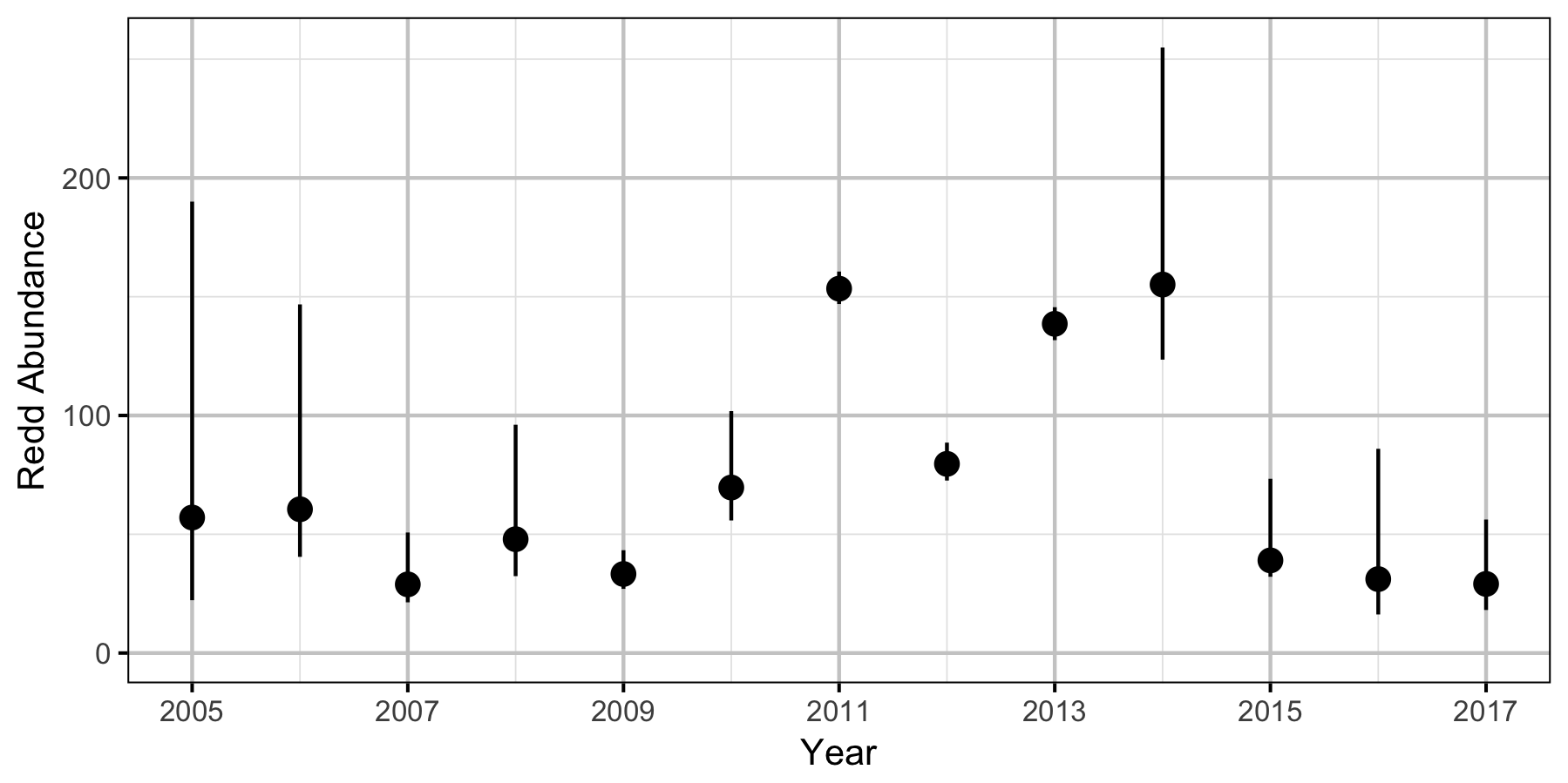
- estimate the abundance of Gerrard Rainbow Trout redds in the tailout area below Duncan Dam;
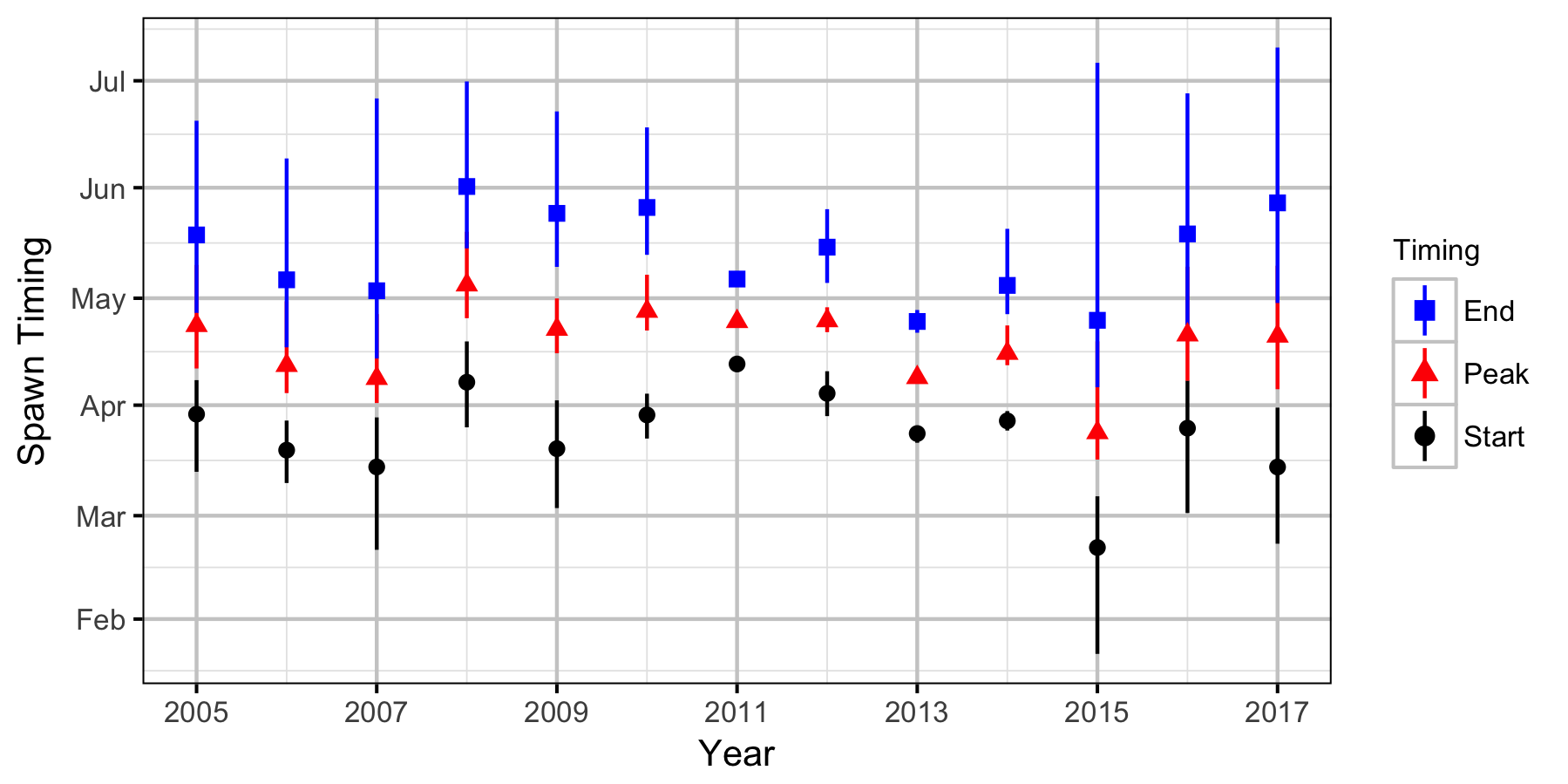
- estimate the spawn timing for the fish utilizing the tailout area;
- estimate the number of redds dewatered.
Data Preparation
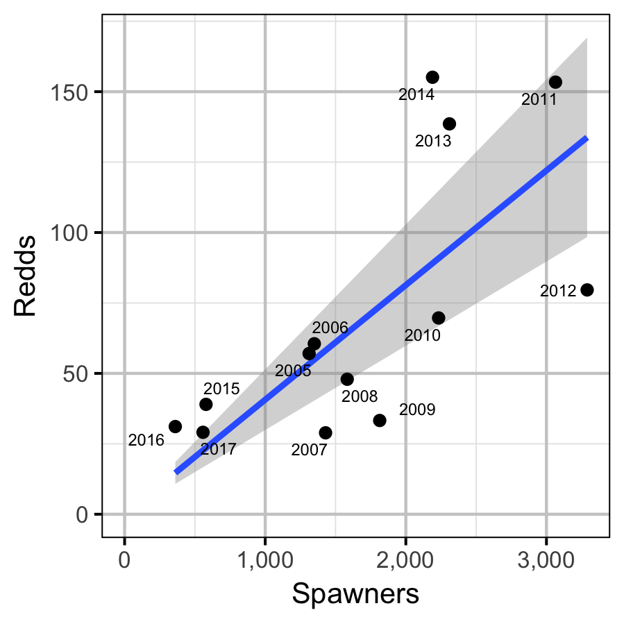
The data were provided by BC Hydro, Ministry of Forests, Lands and Natural Resource Operations, Water Survey of Canada and Mountain Waters Research. The data were prepared for analysis using R version 3.4.4 (R Core Team 2017). The total spawner abundance at Gerrard was assumed to be the observed peak spawner count multiplied 3.08 (Irvine 1978).
Statistical Analysis
Model parameters were estimated using Bayesian methods (McElreath 2016).
Unless indicated otherwise, the Bayesian analyses used uninformative normal prior distributions (Kery and Schaub 2011, 36). The posterior distributions were estimated from 1500 Markov Chain Monte Carlo (MCMC) samples thinned from the second halves of 3 chains (Kery and Schaub 2011, 38–40). Model convergence was confirmed by ensuring that \(\hat{R} \leq 1.1\) (Kery and Schaub 2011, 40) and \(\textrm{ESS} \geq 150\) for each of the monitored parameters (Kery and Schaub 2011, 61). Where \(\hat{R}\) is the potential scale reduction factor and \(\textrm{ESS}\) is the effective sample size.
The parameters are summarised in terms of the point estimate, standard deviation (sd), the z-score, lower and upper 95% credible limits (CLs) and the p-value (Kery and Schaub 2011, 37, 42). The estimate is the median (50th percentile) of the MCMC samples, the z-score is \(\mathrm{mean}/\mathrm{sd}\) and the 95% CLs are the 2.5th and 97.5th percentiles. A p-value of 0.05 indicates that the lower or upper 95% CL is 0.
Where relevant, model adequacy was confirmed by examination of residual plots for the full model(s).
The results are displayed graphically by plotting the modeled relationships between particular variables and the response(s) with the remaining variables held constant. In general, continuous and discrete fixed variables are held constant at their mean and first level values, respectively, while random variables are held constant at their typical values (expected values of the underlying hyperdistributions) (Kery and Schaub 2011, 77–82). When informative the influence of particular variables is expressed in terms of the effect size (i.e., percent change in the response variable) with 95% confidence/credible intervals (CIs, Bradford, Korman, and Higgins 2005).
The analyses were implemented using R version 3.4.4
(R Core Team 2017), JAGS (Plummer 2015), and the
mbr family of packages.
Model Descriptions
Redd Surveys
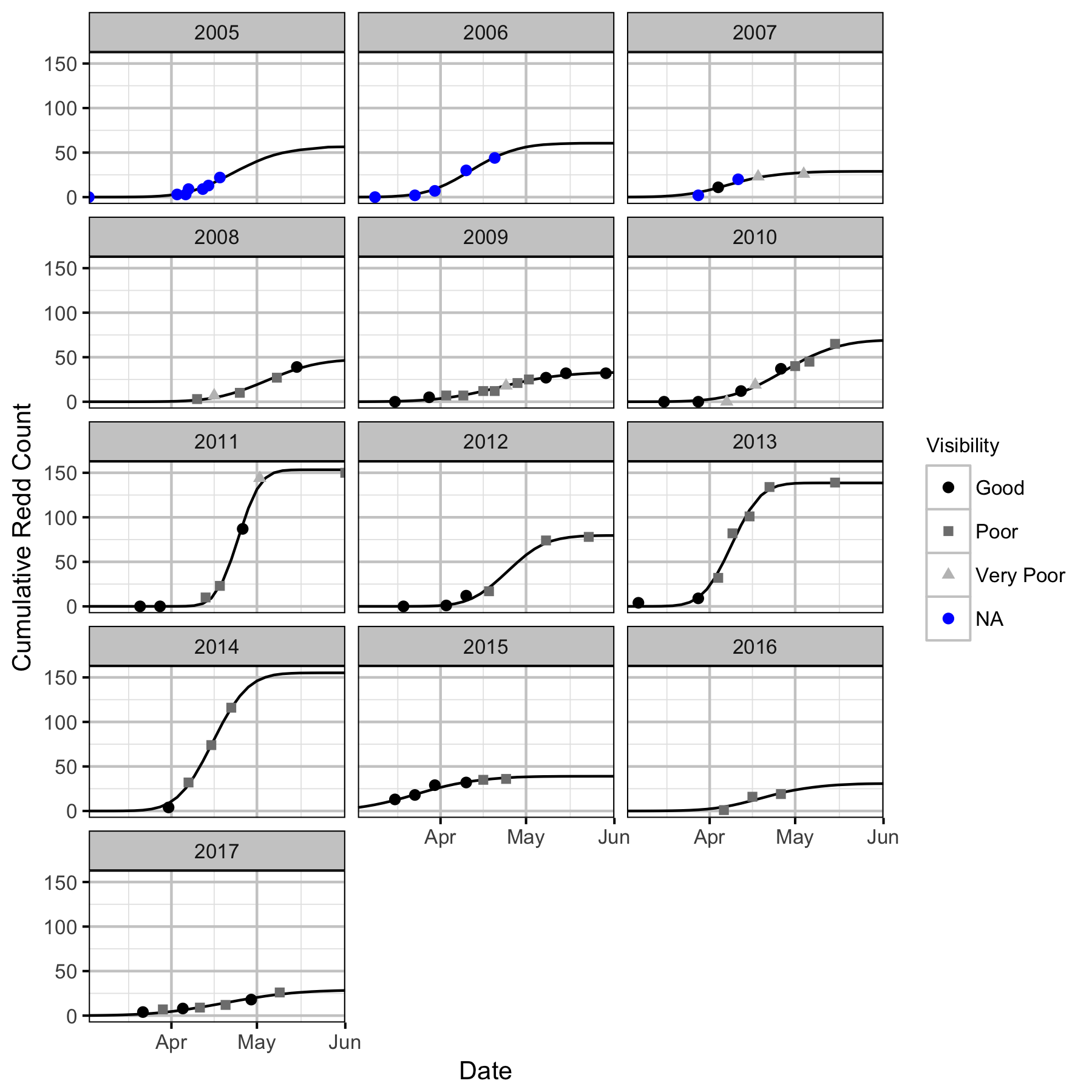
The redd survey counts under surveyable conditions (visibility > 0.6 m) were analysed using a hierarchical Bayesian Area-Under-the-Curve (AUC) model (Hilborn, Bue, and Sharr 1999; Su, Adkison, and Van Alen 2001).
Key assumptions of this model include:
- Observer efficiency is 100%.
- Redd residence time is greater than one month (the maximum time between surveys).
- Spawner abundance varies randomly by year.
- Spawning duration varies randomly by year.
- Spawn timing varies randomly by year.
- The cumulative redd count is normally distributed.
Redd Dewatering
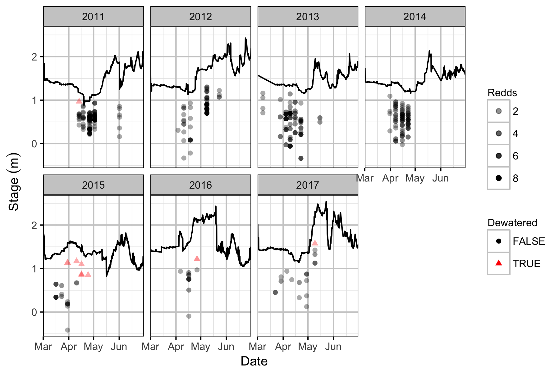
The actual DAL stage heights were compared to the recorded redd elevations. The relative redd elevations were calculated by subtracting the depth of each redd from the stage height at the time the redd depth was recorded.
Key assumptions of this calculation include:
- A redd is dewatered whenever the predicted DAL stage drops below the redds’ relative elevation.
- Emergence occurs at the end of June each year.
Model Templates
Redd Surveys
model{
    bAbundance ~ dnorm(0, 5^-2)
    bTiming ~ dunif(70, 140)
    bDuration ~ dunif(7, 28)

    sAbundanceYear ~ dunif(0, 5)
    sTimingYear ~ dunif(0, 40)
    sDurationYear ~ dunif(0, 20)
    for(i in 1:nYear){
      bTimingYear[i] ~ dnorm (0, sTimingYear^-2)
      bAbundanceYear[i] ~ dnorm (0, sAbundanceYear^-2)
      bDurationYear[i] ~ dnorm (0, sDurationYear^-2)
    }

    sRedds ~ dunif(0, 20)
    for(i in 1:nObs){
      log(eAbundance[i]) <- bAbundance + bAbundanceYear[Year[i]]
      eTiming[i] <- bTiming + bTimingYear[Year[i]]
      eDuration[i] <- bDuration + bDurationYear[Year[i]]

      eRedds[i] <- phi((Doy[i] - eTiming[i]) / eDuration[i]) * eAbundance[i]
      Redds[i] ~ dnorm(eRedds[i], sRedds^-2)
    }
  }
Template 1. The model description.
Results
Tables
Redd Surveys
Table 1. Parameter descriptions.
| Parameter | Description |
|---|---|
| bAbundance | Intercept for eAbundance |
| bAbundanceYear[i] Ef | fect of ith Year on bAbundance |
| bDuration | Intercept for eDuration |
| bDurationYear[i] Ef | fect of ith Year on bDuration |
| bTiming | Intercept for eTiming |
| bTimingYear[i] Ef | fect of ith Year on bTiming |
| Doy[i] Da | y of the year of ith survey |
| eAbundance[i] Ex | pected total cumulative redd count in the ith Year |
| eDuration[i] Ex | pected SD for the duration of spawning for ith survey |
| eRedds[i] Ex | pected cumulative redd count on the ith survey |
| eTiming[i] Ex | pected peak timing of the ith survey |
| Redds[i] Cu | mulative redd count on the ith survey |
| sAbundanceYear | SD of bAbundanceYear |
| sDurationYear | SD of bDurationYear |
| sRedds | SD of residual variation about eRedds |
| sTimingYear | SD of bTimingYear |
| Year[i] Ye | ar of ith survey |
Table 2. Model coefficients.
| term | estimate | sd | zscore | lower | upper | pvalue |
|---|---|---|---|---|---|---|
| bAbundance | 4.097766 | 0.2384242 | 17.192075 | 3.6147698 | 4.559933 | 7e-04 |
| bDuration | 13.175263 | 2.9076779 | 4.662641 | 9.1325248 | 20.786795 | 7e-04 |
| bTiming | 109.783425 | 4.5357696 | 24.200132 | 100.9568936 | 119.407397 | 7e-04 |
| sAbundanceYear | 0.709550 | 0.1895057 | 3.900325 | 0.4518339 | 1.192033 | 7e-04 |
| sDurationYear | 5.389518 | 2.7654778 | 2.160457 | 2.2474155 | 13.413146 | 7e-04 |
| sRedds | 3.879193 | 0.4147368 | 9.440992 | 3.2403727 | 4.819841 | 7e-04 |
| sTimingYear | 12.263854 | 3.6444787 | 3.496405 | 7.0625535 | 21.219208 | 7e-04 |
Table 3. Model summary.
| n | K | nchains | niters | nthin | ess | rhat | converged |
|---|---|---|---|---|---|---|---|
| 83 | 7 | 3 | 500 | 500 | 390 | 1.01 | TRUE |
Table 4. Coefficient table for the linear regression of redd abundance in the tailout on spawner abundance at Gerrard.
| term | estimate | std.error | statistic | p.value |
|---|---|---|---|---|
| Spawners | 0.0406722 | 0.004943 | 8.22821 | 2.8e-06 |
Dewatered
Table 5. The total number of redds counted and the number dewatered based on the stage elevation at DAL.
| Year | Total | Dewatered | Percent |
|---|---|---|---|
| 2011 | 136 | 1 | 1 |
| 2012 | 78 | 0 | 0 |
| 2013 | 140 | 0 | 0 |
| 2014 | 116 | 0 | 0 |
| 2015 | 36 | 7 | 19 |
| 2016 | 19 | 2 | 11 |
| 2017 | 26 | 1 | 4 |
Figures
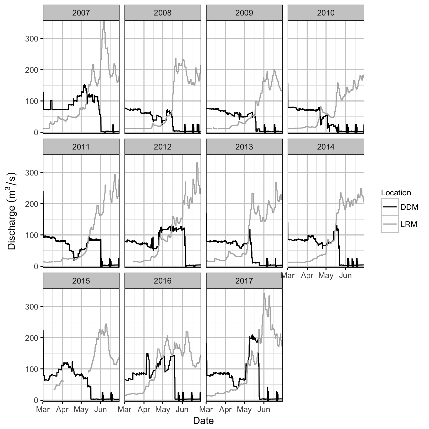
Discharge
Redd Surveys
Acknowledgements
The organisations and individuals whose contributions have made this analysis report possible include:
- BC Hydro
- James Baxter
- Doug Johnson
- Len Wiens
- Kris Wiens
- Ron Greenlaw
- Ministry of Environment
- Jeff Burrows
- Matt Neufeld
- Sarah Stephenson
- Mountain Water Research
- Jeremy Baxter
- Poisson Consulting Ltd.
- Robyn Irvine
- Additional Support
- Clint Tarala
References
Bradford, Michael J, Josh Korman, and Paul S Higgins. 2005. “Using Confidence Intervals to Estimate the Response of Salmon Populations (Oncorhynchus Spp.) to Experimental Habitat Alterations.” Canadian Journal of Fisheries and Aquatic Sciences 62 (12): 2716–26. https://doi.org/10.1139/f05-179.
Hilborn, Ray, Brian G Bue, and Samuel Sharr. 1999. “Estimating Spawning Escapements from Periodic Counts: A Comparison of Methods.” Canadian Journal of Fisheries and Aquatic Sciences 56 (5): 888–96. https://doi.org/10.1139/f99-013.
Irvine, J. R. 1978. “The Gerrard Rainbow Trout of Kootenay Lake, British Columbia - A Discussion of Their Life History with Management, Research and Enhancement Recommendations.” Fisheries Management Report 72. Victoria, BC: Fish; Wildlife Branch.
Kery, Marc, and Michael Schaub. 2011. Bayesian Population Analysis Using WinBUGS : A Hierarchical Perspective. Boston: Academic Press. http://www.vogelwarte.ch/bpa.html.
McElreath, Richard. 2016. Statistical Rethinking: A Bayesian Course with Examples in R and Stan. Chapman & Hall/CRC Texts in Statistical Science Series 122. Boca Raton: CRC Press/Taylor & Francis Group.
Plummer, Martyn. 2015. “JAGS Version 4.0.1 User Manual.” http://sourceforge.net/projects/mcmc-jags/files/Manuals/4.x/.
R Core Team. 2017. “R: A Language and Environment for Statistical Computing.” Vienna, Austria: R Foundation for Statistical Computing. https://www.R-project.org/.
Su, Zhenming, Milo D. Adkison, and Benjamin W. Van Alen. 2001. “A Hierarchical Bayesian Model for Estimating Historical Salmon Escapement and Escapement Timing.” Canadian Journal of Fisheries and Aquatic Sciences 58 (8): 1648–62. https://doi.org/10.1139/cjfas-58-8-1648.