Lower Duncan River Kokanee AUC Analysis 2015
The suggested citation for this analytic report is:
Thorley, J.L. and Hogan, P.M. (2015) Lower Duncan River Kokanee AUC Analysis 2015. A Poisson Consulting Analysis Report. URL: https://www.poissonconsulting.ca/f/1629724501.
Background
Since 2008 aerial surveys have been conducted in the Lower Duncan River (LDR) to count the number of kokanee spawners. The primary objectives of the current analysis report are to:
- Estimate the aerial observer efficiency based on ground counts.
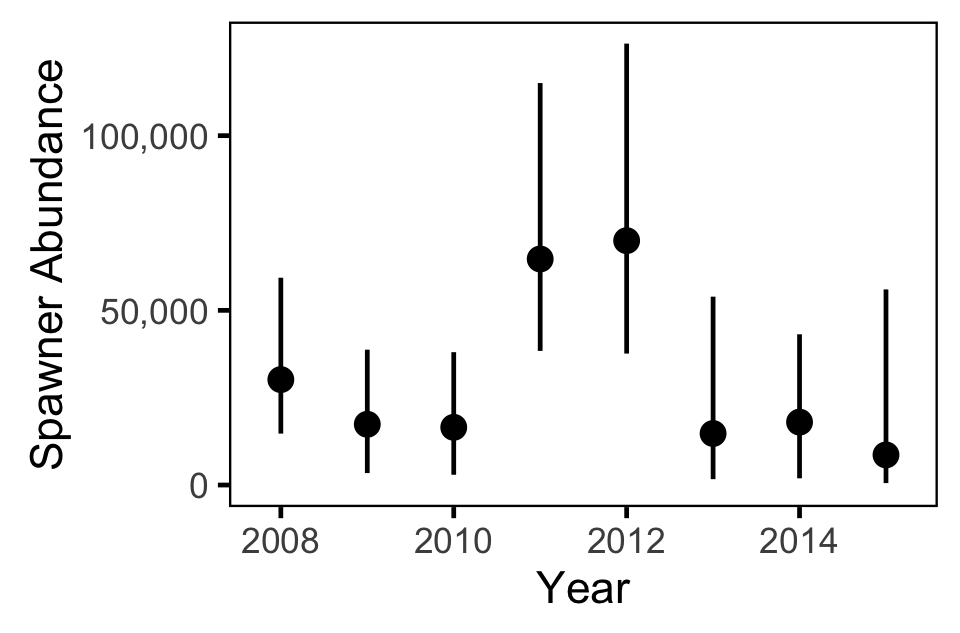
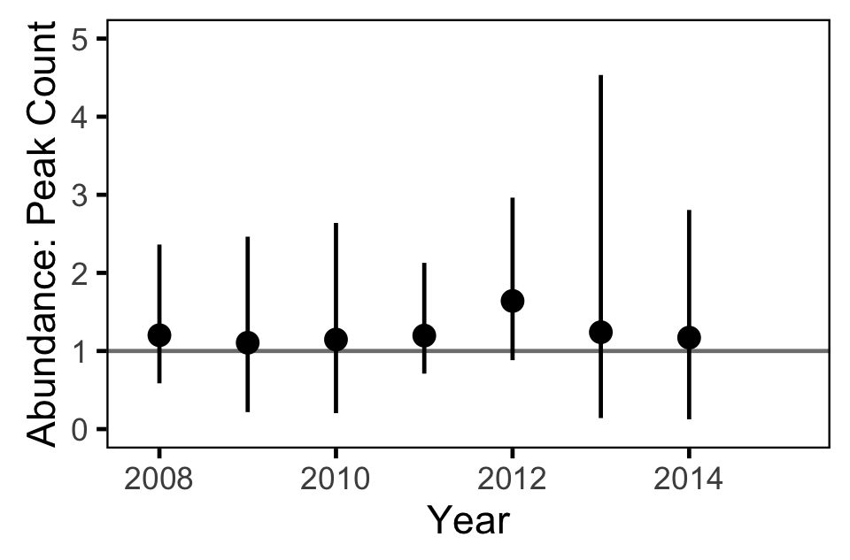
- Estimate the annual kokanee spawner abundance from the aerial counts.
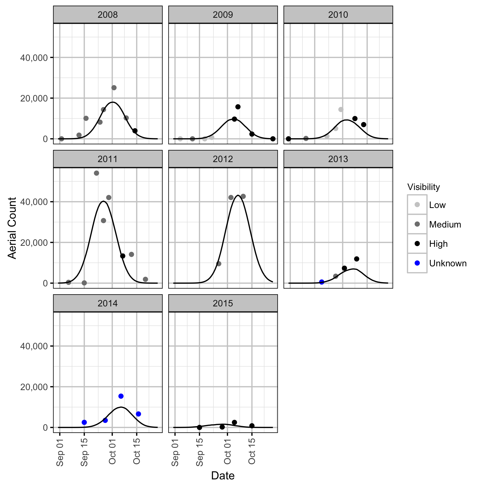
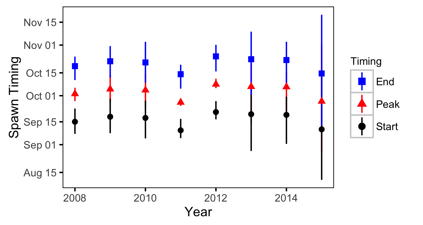
- Estimate the peak spawn timing.
Methods
Data Preparation
The data were provided by LGL Limited in the form of an Access database and an Excel spreadsheet.
Statistical Analysis
Hierarchical Bayesian models were fitted to the count data using R version 3.2.3 (Team 2013) and JAGS 4.0.1 (Plummer 2015) which interfaced with each other via jaggernaut 2.3.1 (Thorley 2013). For additional information on hierarchical Bayesian modelling in the BUGS language, of which JAGS uses a dialect, the reader is referred to (Kery and Schaub 2011, 41–44).
Unless specified, the models assumed vague (low information) prior distributions (Kery and Schaub 2011, 36). The posterior distributions were estimated from a minimum of 1,000 Markov Chain Monte Carlo (MCMC) samples thinned from the second halves of three chains (Kery and Schaub 2011, 38–40). Model convergence was confirmed by ensuring that Rhat (Kery and Schaub 2011, 40) was less than 1.1 for each of the parameters in the model (Kery and Schaub 2011, 61).
The posterior distributions of the fixed (Kery and Schaub 2011, 75) parameters are summarised in terms of a point estimate (median), lower and upper 95% credible limits (2.5th and 97.5th percentiles), the standard deviation (SD), percent relative error (half the 95% credible interval as a percent of the point estimate) and significance (Kery and Schaub 2011, 37, 42).
Variable selection was achieved by dropping insignificant (Kery and Schaub 2011, 37, 42) fixed (Kery and Schaub 2011, 77–82) variables and uninformative random variables. A fixed variables was considered to be insignificant if its significance was \(\geq\) 0.05 while a random variable was considered to be uninformative if its percent relative error was \(\geq\) 80%. The Deviance Information Criterion (DIC) was not used because it is of questionable validity when applied to hierarchical models (Kery and Schaub 2011, 469).
The results are displayed graphically by plotting the modelled relationships between particular variables and the response with 95% credible intervals (CRIs) with the remaining variables held constant. In general, continuous and discrete fixed variables are held constant at their mean and first level values respectively while random variables are held constant at their typical values (expected values of the underlying hyperdistributions) (Kery and Schaub 2011, 77–82). Where informative the influence of particular variables is expressed in terms of the effect size (i.e., percent change in the response variable) with 95% CRIs (Bradford, Korman, and Higgins 2005).
Observer Efficiency
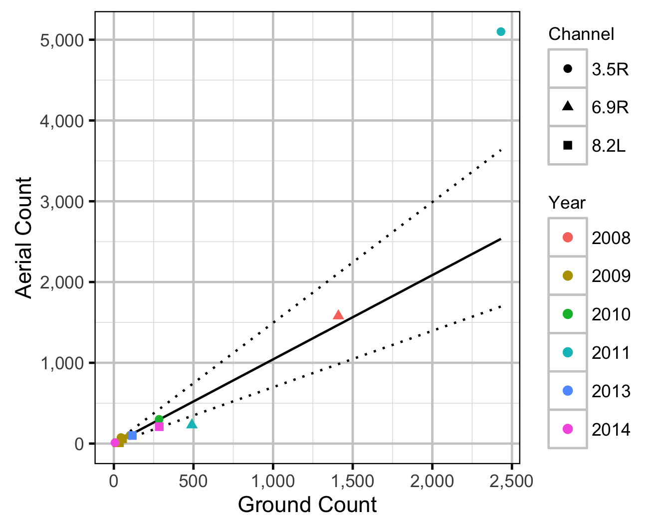
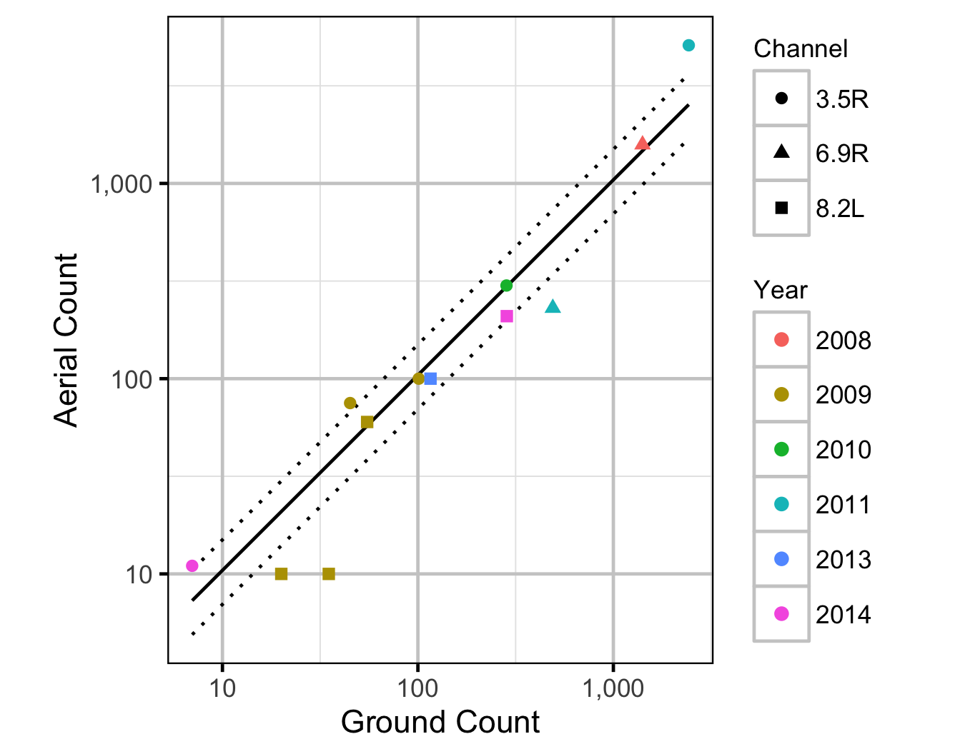
The aerial observer efficiency was estimated from ground counts using a Poisson model. Key assumptions of the observer efficiency model include:
- Spawner abundance at a site does not vary between the ground and aerial count.
- Ground observers are unbiased.
- Ground counts are drawn from a Poisson distribution.
- Aerial counts are drawn from an overdispersed Poisson distribution.
- Aerial observer efficiency does not vary with abundance or channel type (side versus main channel).
Area-Under-the-Curve
The aerial spawner counts were analysed using a hierarchical Bayesian Area-Under-the-Curve (AUC) model (Hilborn, Bue, and Sharr 1999). Key assumptions of the AUC model include:
- Spawner arrival and departure times are normally distributed (Hilborn, Bue, and Sharr 1999).
- Spawner duration is constant across years.
- Spawner abundance varies randomly by year, drawn from a normal distribution.
- Peak spawn timing varies randomly by year, drawn from a normal distribution (Su, Adkison, and Van Alen 2001).
- Spawner residence time is between 7 and 14 days (Acara 1970, @morbey_timing_2003).
- Spawner observer efficiency is drawn from a normal distribution as estimated by the observer efficiency model, with a mean of 1.05, SD of 0.15 and lower and upper limits of 0.79 and 1.36 respectively.
- The residual variation in the spawner counts is normally distributed.
Model Code
The JAGS model code, which uses a series of naming conventions, is presented below.
Observer Efficiency
| Variable/Parameter | Description |
|---|---|
Aerial[i] |
Aerial count for ith survey |
bAbundance |
log(eAbundance) intercept |
bEfficiency |
eEfficiency intercept |
eAbundance[i] |
Expected spawner abundance for ith survey |
eAerial[i] |
Expected aerial count for ith survey |
eEfficiency[i] |
Expected aerial observer efficiency for ith survey |
Ground[i] |
Ground count for ith survey |
sAbundance |
SD of residual variation in log(eAbundance) |
sDispersion |
SD of overdispersion |
Observer Efficiency - Model1
model{

  bEfficiency ~ dunif(0, 3)

  bAbundance ~ dnorm(5, 5^-2)
  sAbundance ~ dunif(0, 5)

  sDispersion ~ dunif(0, 5)
  for (i in 1:length(Aerial)){

    eEfficiency[i] <- bEfficiency

    eAbundance[i] ~ dlnorm(bAbundance, sAbundance^-2)
    Ground[i] ~ dpois(eAbundance[i])

    eAerial[i] <- eAbundance[i] * eEfficiency[i]
    eDispersion[i] ~ dgamma(1 / sDispersion^2, 1 / sDispersion^2)
    Aerial[i] ~ dpois(eAerial[i] * eDispersion[i])
  }
}
Area-Under-The-Curve
| Variable/Parameter | Description |
|---|---|
bAbundance |
log(eAbundance) intercept |
bAbundanceYear[i] |
Effect of ith year on log(eAbundance) |
bDuration |
eDuration intercept |
bEfficiency |
eEfficiency intercept |
bPeakTiming |
ePeakTiming intercept |
bPeakTimingYear[i] |
Effect of ith year on ePeakTiming |
bResidenceTime |
Spawner residence time |
Count[i] |
Spawner count for ith survey |
Dayte[i] |
Centred day of the year for ith survey |
eAbundance[i] |
Expected annual spawner abundance for ith survey |
eCount[i] |
Expected spawner count for ith survey |
eDuration[i] |
Expected SD of the duration of spawner arrival timing |
eEfficiency[i] |
Expected aerial observer efficiency for ith survey |
ePeakTiming[i] |
Expected timing of annual peak spawner abundance for ith survey |
eSpawners[i] |
Expected number of spawners for ith survey |
sAbundanceYear |
SD of effect of year on log(eAbundance) |
sCount |
SD of residual variation in eCount |
sPeakTimingYear |
SD of effect of year on ePeakTiming |
Area-Under-The-Curve - Model1
model{

  bEfficiency ~ dnorm(1.05, 0.15^-2) T(0.79, 1.36)

  bAbundance ~ dnorm(10, 5^-2)
  bPeakTiming ~ dnorm(0, 5)
  bDuration ~ dunif(0, 42)

  sAbundanceYear ~ dunif(0, 5)
  sPeakTimingYear ~ dunif(0, 28)
  for(i in 1:nYear){
    bAbundanceYear[i] ~ dnorm(0, sAbundanceYear^-2)
    bPeakTimingYear[i] ~ dnorm(0, sPeakTimingYear^-2)
  }

  bResidenceTime ~ dunif(7, 14)

  sCount ~ dunif(0, 10000)
  for(i in 1:length(Count)){

    log(eAbundance[i]) <- bAbundance + bAbundanceYear[Year[i]]

    ePeakTiming[i] <- bPeakTiming + bPeakTimingYear[Year[i]]

    eDuration[i] <- bDuration

    eSpawners[i] <- ( phi((Dayte[i] - (ePeakTiming[i] - bResidenceTime/2)) / eDuration[i])
                     -phi((Dayte[i] - (ePeakTiming[i] + bResidenceTime/2)) / eDuration[i])
                    ) * eAbundance[i]

    eEfficiency[i] <- bEfficiency

    eCount[i] <- eSpawners[i] * eEfficiency[i]
    Count[i] ~ dnorm(eCount[i], sCount^-2)
  }
}
Results
Model Parameters
The posterior distributions for the fixed (Kery and Schaub 2011 p. 75) parameters in each model are summarised below.
Observer Efficiency
| Parameter | Estimate | Lower | Upper | SD | Error | Significance |
|---|---|---|---|---|---|---|
| bAbundance | 4.8610 | 3.8450 | 5.9600 | 0.5580 | 22 | 0.001 |
| bEfficiency | 1.0607 | 0.6980 | 1.4954 | 0.2003 | 38 | 0.001 |
| sAbundance | 1.9720 | 1.2510 | 3.0790 | 0.4850 | 46 | 0.001 |
| sDispersion | 0.5569 | 0.3555 | 0.8776 | 0.1419 | 47 | 0.001 |
| Convergence | Iterations |
|---|---|
| 1.05 | 20000 |
Area-Under-The-Curve
| Parameter | Estimate | Lower | Upper | SD | Error | Significance |
|---|---|---|---|---|---|---|
| bAbundance | 9.9900 | 8.8160 | 10.9470 | 0.5540 | 11 | 0.0010 |
| bDuration | 5.8400 | 1.2960 | 8.3460 | 1.6640 | 60 | 0.0010 |
| bEfficiency | 1.0578 | 0.8253 | 1.3204 | 0.1308 | 23 | 0.0010 |
| bPeakTiming | 0.0980 | -0.7690 | 0.9430 | 0.4480 | 870 | 0.8104 |
| bResidenceTime | 10.9840 | 7.2900 | 13.8860 | 2.0560 | 30 | 0.0010 |
| sAbundanceYear | 1.1540 | 0.4640 | 2.8230 | 0.6050 | 100 | 0.0010 |
| sCount | 5965.0000 | 4651.0000 | 7595.0000 | 780.0000 | 25 | 0.0010 |
| sPeakTimingYear | 10.8000 | 4.7200 | 23.4200 | 4.8400 | 87 | 0.0010 |
| Convergence | Iterations |
|---|---|
| 1.04 | 10000 |
Figures
Observer Efficiency
Area-Under-The-Curve
Acknowledgements
The organisations and individuals whose contributions have made this analysis report possible include:
- BC Hydro
- Guy Martel
- Okanagan National Alliance
- Michael Zimmer
- Natasha Audy
- Skyeler Folks
- LGL Limited
- Elmar Plate
- Amec Earth and Environmental
- Louise Porto
- Crystal Lawrence
- Clint Tarala
- Poisson Consulting Ltd.
- Robyn Irvine
References
Acara, A. H. 1970. “The Meadow Creek Spawning Channel. Unpublished Report.” Victoria, BC: Fish; Wildlife Branch.
Bradford, Michael J, Josh Korman, and Paul S Higgins. 2005. “Using Confidence Intervals to Estimate the Response of Salmon Populations (Oncorhynchus Spp.) to Experimental Habitat Alterations.” Canadian Journal of Fisheries and Aquatic Sciences 62 (12): 2716–26. https://doi.org/10.1139/f05-179.
Hilborn, Ray, Brian G Bue, and Samuel Sharr. 1999. “Estimating Spawning Escapements from Periodic Counts: A Comparison of Methods.” Canadian Journal of Fisheries and Aquatic Sciences 56 (5): 888–96. https://doi.org/10.1139/f99-013.
Kery, Marc, and Michael Schaub. 2011. Bayesian Population Analysis Using WinBUGS : A Hierarchical Perspective. Boston: Academic Press. http://www.vogelwarte.ch/bpa.html.
Morbey, Y. E., and R. C. Ydenberg. 2003. “Timing Games in the Reproductive Phenology of Female Pacific Salmon (Oncorhynchus Spp.).” The American Naturalist 161 (2): 284–98. http://www.jstor.org/stable/10.1086/345785.
Plummer, Martyn. 2015. “JAGS Version 4.0.1 User Manual.” http://sourceforge.net/projects/mcmc-jags/files/Manuals/4.x/.
Su, Zhenming, Milo D. Adkison, and Benjamin W. Van Alen. 2001. “A Hierarchical Bayesian Model for Estimating Historical Salmon Escapement and Escapement Timing.” Canadian Journal of Fisheries and Aquatic Sciences 58 (8): 1648–62. https://doi.org/10.1139/cjfas-58-8-1648.
Team, R Core. 2013. “R: A Language and Environment for Statistical Computing.” Vienna, Austria: R Foundation for Statistical Computing. http://www.R-project.org.
Thorley, J. L. 2013. “Jaggernaut: An R Package to Facilitate Bayesian Analyses Using JAGS (Just Another Gibbs Sampler).” Nelson, B.C.: Poisson Consulting Ltd. https://github.com/poissonconsulting/jaggernaut.