Lower Duncan River Kokanee AUC Analysis 2017
The suggested citation for this analytic report is:
Thorley, J.L. (2018) Lower Duncan River Kokanee AUC Analysis 2017. A Poisson Consulting Analysis Report. URL: https://www.poissonconsulting.ca/f/1498798685.
Background
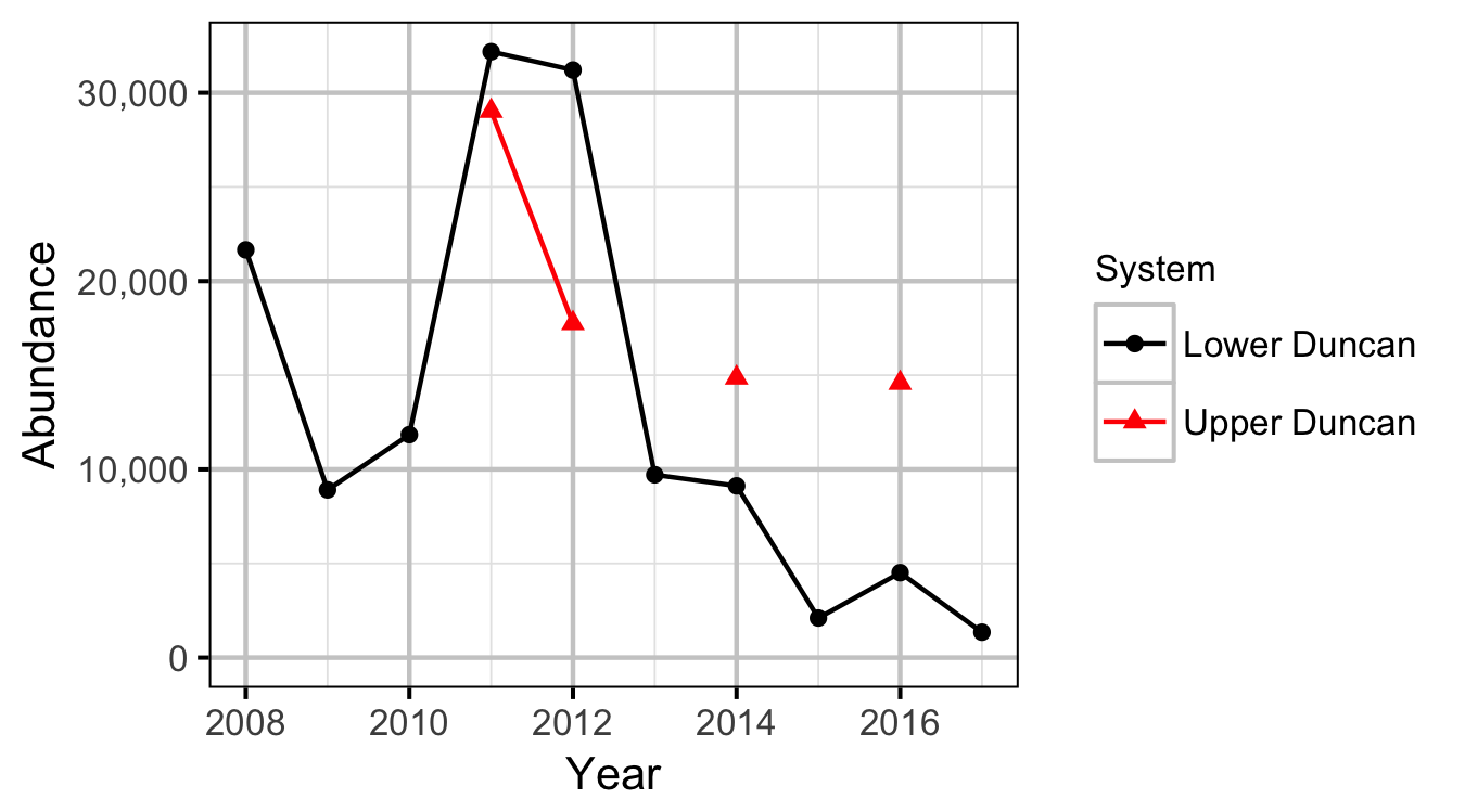
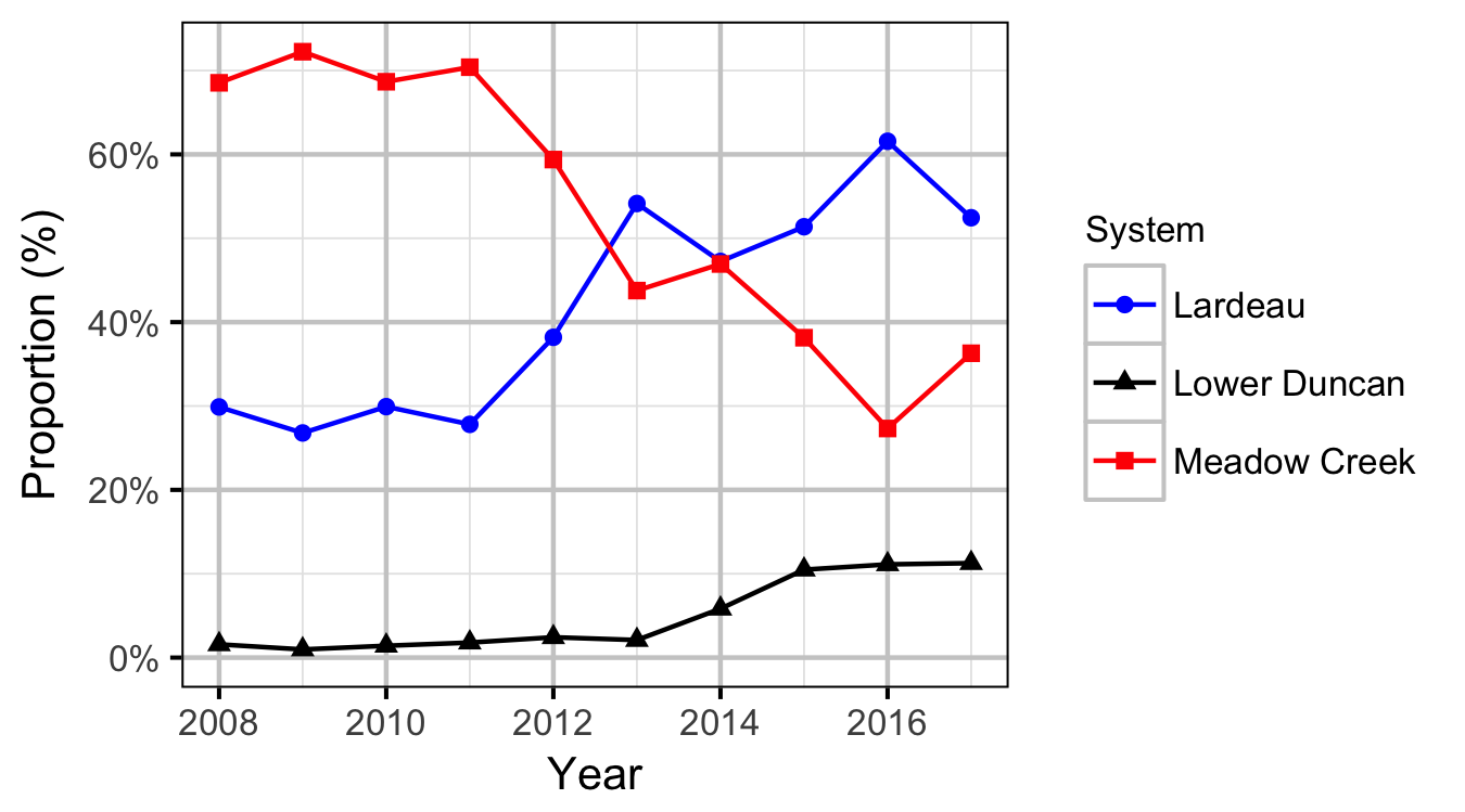
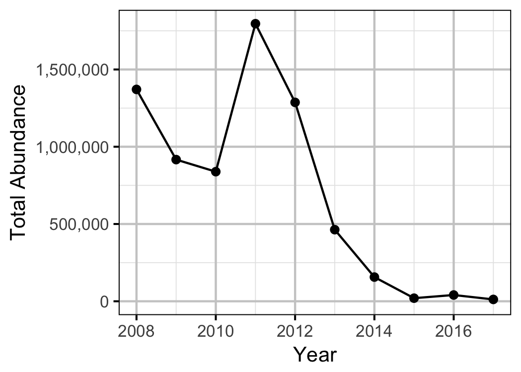
Every fall, Kokanee from Kootenay Lake spawn in the Duncan-Lardeau system. Since 2008 aerial surveys have been conducted in the Lower Duncan River (LDR) to enumerate the number of kokanee spawners. The management questions are:
- What is the spawn run timing, fry emergence timing, and relative intensity of kokanee spawning in the Lower Duncan River? What potential operational/environmental cues affect this variable?
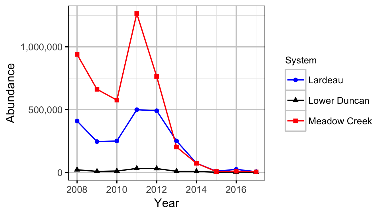
- What are the timing/cues of kokanee spawners in Meadow Creek and Lardeau River systems?
- What are the relative distribution of kokanee spawners in the Lower Duncan River, Meadow Creek and Lardeau River? What potential operation/environmental/physical cues (e.g., temperature, velocity, depth, cover, substrate) affect this variable?; and
- What physical works or operational constraints could be implemented to minimize operational conflicts associated with recommended kokanee spawning operations?
Data Preparation
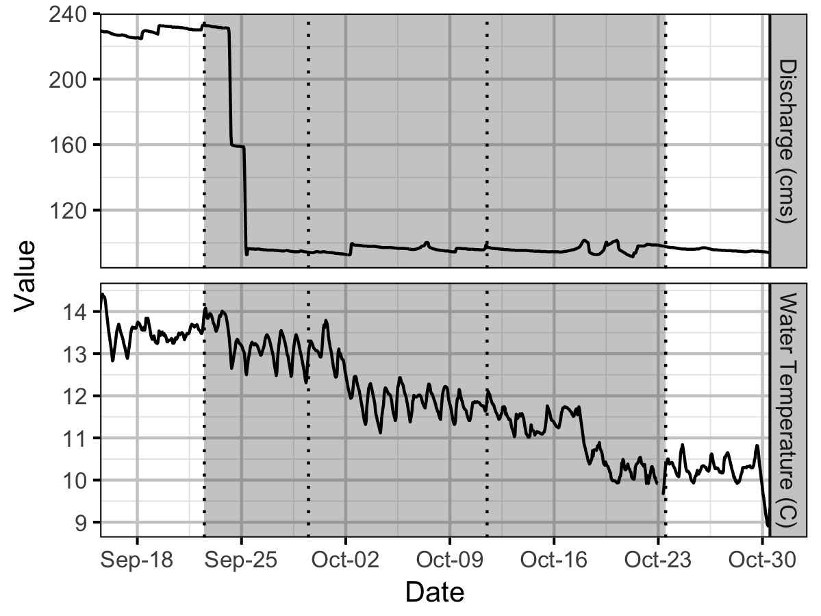
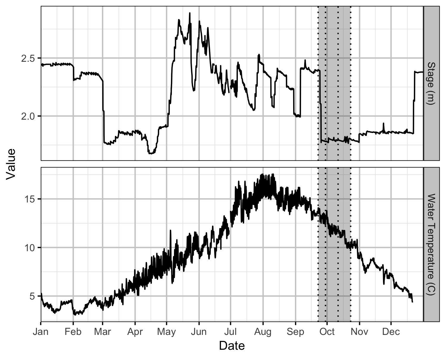
The 2017 survey data were provided by LGL Limited in the form of Excel tables. They were imported into the existing SQLite database. The data were clean and tidied (Wickham 2014) using R version 3.4.3 (R Core Team 2016). When there were repeated counts for a channel the higher of the two values was choosen. The mean daily discharge and water temperature values at Duncan River below Lardeau (DRL) were extracted from BC Hydro’s environmental database for the Kootenays, which is maintained by Poisson Consulting. The annual abundances of Kokanee spawning in Meadow Creek and the Lardeau River were provided by the Ministry of Forests, Lands and Natural Resource Operations.
Statistical Analysis
Model parameters were estimated using Bayesian methods. The estimates were produced using JAGS (Plummer 2015). For additional information on Bayesian estimation the reader is referred to McElreath (2016).
Unless indicated otherwise, the Bayesian analyses used uninformative normal prior distributions (Kery and Schaub 2011, 36). The posterior distributions were estimated from 1500 Markov Chain Monte Carlo (MCMC) samples thinned from the second halves of 3 chains (Kery and Schaub 2011, 38–40). Model convergence was confirmed by ensuring that \(\hat{R} \leq 1.1\) (Kery and Schaub 2011, 40) and \(\textrm{ESS} \geq 150\) for each of the monitored parameters (Kery and Schaub 2011, 61). Where \(\hat{R}\) is the potential scale reduction factor and \(\textrm{ESS}\) is the effective sample size.
The parameters are summarised in terms of the point estimate, standard deviation (sd), the z-score, lower and upper 95% confidence/credible limits (CLs) and the p-value (Kery and Schaub 2011, 37, 42). The estimate is the median (50th percentile) of the MCMC samples, the z-score is \(\mathrm{mean}/\mathrm{sd}\) and the 95% CLs are the 2.5th and 97.5th percentiles. A p-value of 0.05 indicates that the lower or upper 95% CL is 0.
Where relevant, model adequacy was confirmed by examination of residual plots for the full model(s).
The results are displayed graphically by plotting the modeled relationships between particular variables and the response(s) with the remaining variables held constant. In general, continuous and discrete fixed variables are held constant at their mean and first level values, respectively, while random variables are held constant at their typical values (expected values of the underlying hyperdistributions) (Kery and Schaub 2011, 77–82). When informative the influence of particular variables is expressed in terms of the effect size (i.e., percent change in the response variable) with 95% confidence/credible intervals (CIs, Bradford, Korman, and Higgins 2005).
The analyses were implemented using R version 3.4.3
(R Core Team 2015) and the
mbr family of packages.
Model Descriptions
Observer Efficiency
The aerial observer efficiency was estimated from ground counts using an overdispersed Poisson regression. Key assumptions of the observer efficiency model include:
- The ground counts are accurate.
- The residual variation in the aerial counts is gamma-Poisson distributed.
Area-Under-the-Curve
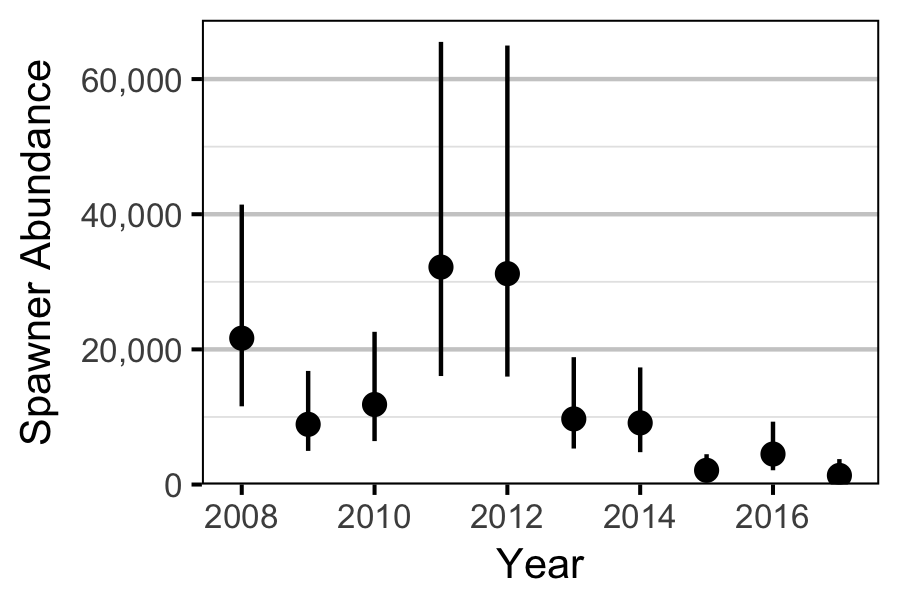
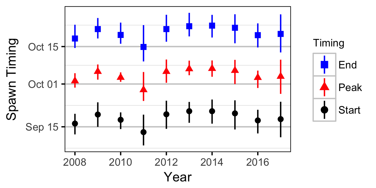
The aerial spawner counts for the Lower Duncan River and its sidechannels were analysed using a hierarchical Bayesian Area-Under-the-Curve (AUC) model (Hilborn, Bue, and Sharr 1999). Key assumptions of the AUC model include:
- Spawner arrival and departure times are normally distributed (Hilborn, Bue, and Sharr 1999).
- Spawner duration is constant across years.
- Spawner abundance varies randomly by year.
- Peak spawn timing varies randomly by year (Su, Adkison, and Van Alen 2001).
- Spawner residence time is between 7 and 14 days (Acara 1970, @morbey_timing_2003).
- Spawner observer efficiency is drawn from a normal distribution as estimated by the observer efficiency model, with a mean of 1.40, SD of 0.38 and lower and upper limits of 0.89 and 2.39 respectively.
- The standard deviation of the residual variation in the spawner counts varies by the annual abundance.
- The residual variation in the spawner counts is normally distributed.
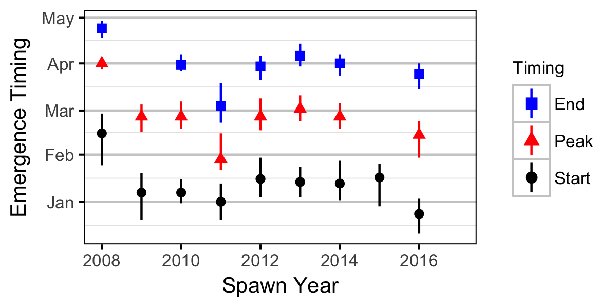
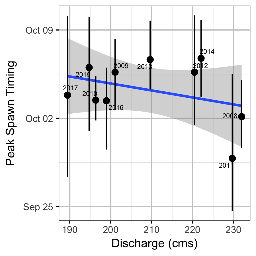
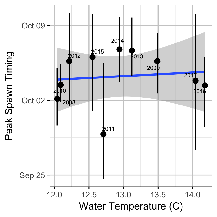
The emergence timing was calculated from the daily water temperature at DRL assuming 950 Accumulated Thermal Units (ATUs). The relationship between peak spawn timing and the mean september water temperature at DRL was tested using linear regression. Neither relationship was significant (p > 0.3).
Model Templates
Observer Efficiency
model{

  bEfficiency ~ dunif(0, 3)
  sDispersion ~ dunif(0, 5)

  for (i in 1:nObs){
    eAerial[i] <- Ground[i] * bEfficiency
    eDispersion[i] ~ dgamma(sDispersion^-2, sDispersion^-2)
    Aerial[i] ~ dpois(eAerial[i] * eDispersion[i])
  }
..
Template 1. Model definition.
Area-Under-The-Curve
model{
  bAbundance ~ dnorm(10, 5^-2)
  bPeakTiming ~ dunif(-14, 14)
  bDuration ~ dnorm(2, 1^-2)

  bEfficiency ~ dnorm(1.40, 0.38^-2) T(0.89, 2.40)
  bResidenceTime ~ dunif(7, 14)

  sAbundanceYear ~ dunif(0, 5)
  sPeakTiming ~ dunif(0, 14)
  for(i in 1:nYear){
    bAbundanceYear[i] ~ dnorm(0, sAbundanceYear^-2)
    bPeakTimingYear[i] ~ dnorm(0, sPeakTiming^-2)
  }

  bSD ~ dnorm(0, 10^-2)
  bSDAbundance ~ dnorm(0, 5^-2)
  for(i in 1:length(Count)){

    log(eAbundance[i]) <- bAbundance + bAbundanceYear[Year[i]]
    ePeakTiming[i] <- bPeakTiming + bPeakTimingYear[Year[i]]
    log(eDuration[i]) <- bDuration

    eArrived[i] <- pnorm(Dayte[i], (ePeakTiming[i] - bResidenceTime/2), eDuration[i]^-2)
    eDeparted[i] <- pnorm(Dayte[i], (ePeakTiming[i] + bResidenceTime/2), eDuration[i]^-2)
    eSpawners[i] <- (eArrived[i] - eDeparted[i]) * eAbundance[i]

    eEfficiency[i] <- bEfficiency

    log(eSD[i]) <- bSD + bSDAbundance * eAbundance[i]

    Count[i] ~ dnorm(eSpawners[i] * eEfficiency[i], eSD[i]^-2)
  }
..
Template 2. Model definition.
Results
Tables
Observer Efficiency
Table 1. Parameter descriptions.
| Parameter | Description |
|---|---|
Aerial[i] |
Aerial count for ith survey |
bEfficiency |
eEfficiency intercept |
eAerial[i] |
Expected aerial count for ith survey |
Ground[i] |
Ground count for ith survey |
sDispersion |
SD of overdispersion |
Table 2. Model coefficients.
| term | estimate | sd | zscore | lower | upper | pvalue |
|---|---|---|---|---|---|---|
| bEfficiency | 1.3987374 | 0.3823003 | 3.832617 | 0.8919527 | 2.397768 | 7e-04 |
| sDispersion | 0.8690359 | 0.1721166 | 5.164291 | 0.6171624 | 1.276703 | 7e-04 |
Table 3. Model summary.
| n | K | nchains | niters | nthin | ess | rhat | converged |
|---|---|---|---|---|---|---|---|
| 15 | 2 | 3 | 500 | 200 | 195 | 1.02 | TRUE |
Table 4.
| Dayte | Year | Channel | Ground | Aerial |
|---|---|---|---|---|
| 1972-09-24 | 2008 | 6.9R | 1484 | 1710 |
| 1972-09-22 | 2009 | 3.5R | 45 | 75 |
| 1972-10-02 | 2009 | 3.5R | 101 | 100 |
| 1972-09-22 | 2009 | 8.2L | 75 | 172 |
| 1972-10-02 | 2009 | 8.2L | 35 | 15 |
| 1972-10-09 | 2009 | 8.2L | 299 | 10 |
| 1972-10-06 | 2010 | 3.5R | 284 | 822 |
| 1972-09-29 | 2011 | 3.5R | 2518 | 5720 |
| 1972-09-29 | 2011 | 6.9R | 490 | 230 |
| 1972-09-27 | 2014 | 3.5R | 7 | 20 |
| 1972-09-27 | 2014 | 8.2L | 285 | 294 |
| 1972-09-23 | 2016 | 3.5R | 3 | 2 |
| 1972-09-23 | 2016 | CAL | 67 | 61 |
| 1972-09-29 | 2016 | CAL | 30 | 29 |
| 1972-09-22 | 2017 | CAL | 4 | 2 |
Channel Count
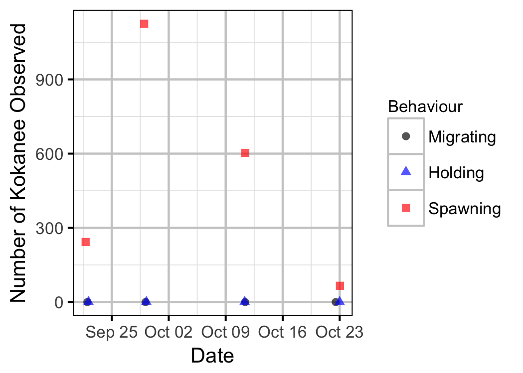
Table 5. Number of observed Kokanee distributed in the LDR main stem and side channels for 2017.
| Date | Channel | Migrating | Holding | Spawning |
|---|---|---|---|---|
| 2017-09-22 | Main | 0 | 0 | 175 |
| 2017-09-22 | Side | 0 | 0 | 68 |
| 2017-09-29 | Main | 0 | 0 | 1105 |
| 2017-09-29 | Side | 0 | 0 | 20 |
| 2017-10-11 | Main | 0 | 0 | 603 |
| 2017-10-11 | Side | 0 | 0 | 0 |
| 2017-10-23 | Main | 0 | 0 | 66 |
| 2017-10-23 | Side | 0 | 0 | 0 |
Area-Under-The-Curve
Table 6. Parameter descriptions.
| Parameter | Description |
|---|---|
bAbundance |
log(eAbundance) intercept |
bAbundanceYear[i] |
Effect of ith year on log(eAbundance) |
bDuration |
eDuration intercept |
bEfficiency |
eEfficiency intercept |
bPeakTiming |
ePeakTiming intercept |
bPeakTimingYear[i] |
Effect of ith year on ePeakTiming |
bResidenceTime |
Spawner residence time |
Count[i] |
Spawner count for ith survey |
Dayte[i] |
Centred day of the year for ith survey |
eAbundance[i] |
Expected annual spawner abundance for ith survey |
eCount[i] |
Expected spawner count for ith survey |
eDuration[i] |
Expected SD of the duration of spawner arrival timing |
eEfficiency[i] |
Expected aerial observer efficiency for ith survey |
ePeakTiming[i] |
Expected timing of annual peak spawner abundance for
ith survey |
eSpawners[i] |
Expected number of spawners for ith survey |
FullYear[i] |
Indicates whether seven or more surveys in ith
year |
sAbundanceYear |
SD of effect of year on log(eAbundance) |
sCount |
SD of residual variation in eCount |
sPeakTiming |
SD of effect of year on ePeakTiming |
Table 7. Model coefficients.
| term | estimate | sd | zscore | lower | upper | pvalue |
|---|---|---|---|---|---|---|
| bAbundance | 9.0683836 | 0.5110704 | 17.750724 | 8.1233442 | 10.1389831 | 7e-04 |
| bDuration | 1.6892354 | 0.1562009 | 10.753932 | 1.3445456 | 1.9681027 | 7e-04 |
| bEfficiency | 1.5184787 | 0.3228957 | 4.745053 | 0.9537047 | 2.1960404 | 7e-04 |
| bPeakTiming | 5.4369435 | 1.3516356 | 3.995801 | 2.6696997 | 8.0230040 | 7e-04 |
| bResidenceTime | 10.8699687 | 1.9879654 | 5.404758 | 7.2094767 | 13.8366737 | 7e-04 |
| bSD | 6.3971805 | 0.4339157 | 14.629159 | 5.3688834 | 7.0451946 | 7e-04 |
| bSDAbundance | 0.0000905 | 0.0000541 | 1.899899 | 0.0000367 | 0.0002467 | 7e-04 |
| sAbundanceYear | 1.1937338 | 0.4130019 | 3.096462 | 0.7339040 | 2.3227421 | 7e-04 |
| sPeakTiming | 3.2113385 | 1.4890858 | 2.288338 | 1.0493521 | 6.9305643 | 7e-04 |
Table 8. Model summary.
| n | K | nchains | niters | nthin | ess | rhat | converged |
|---|---|---|---|---|---|---|---|
| 55 | 9 | 3 | 500 | 100 | 246 | 1.022 | TRUE |
Figures
Environmental
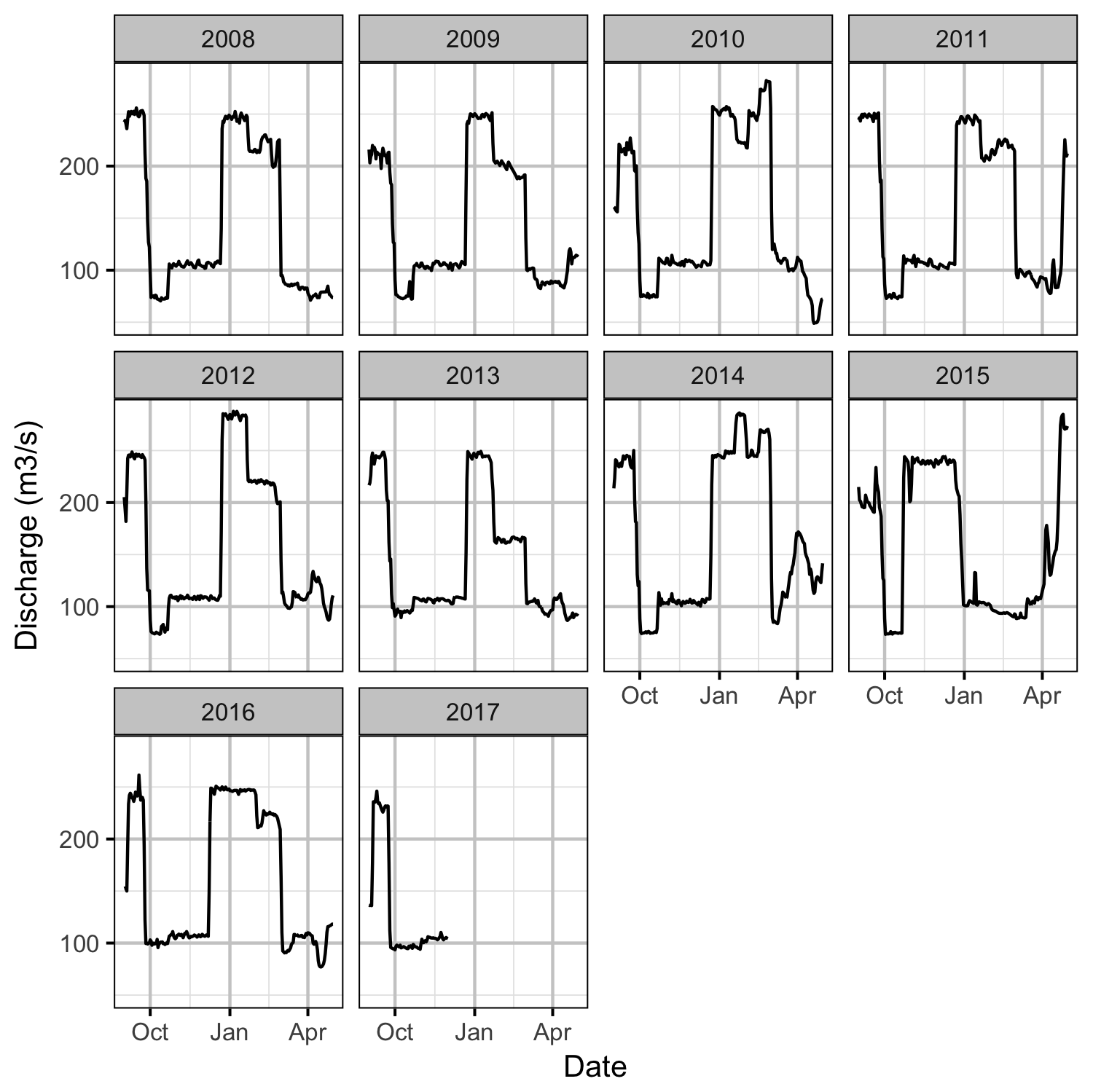
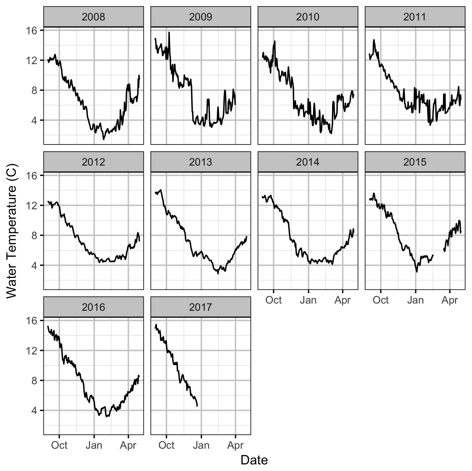
Observer Efficiency
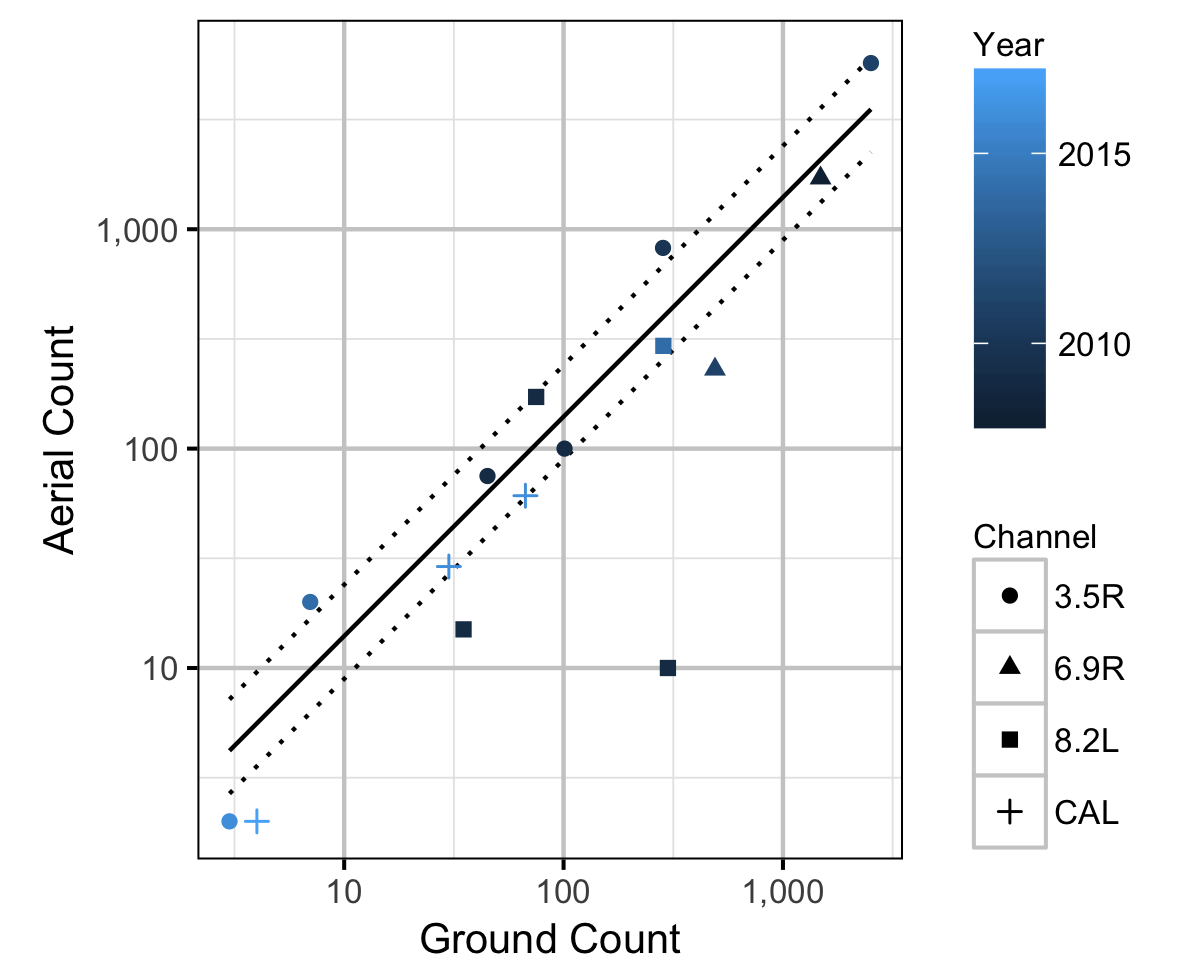
Area-Under-The-Curve
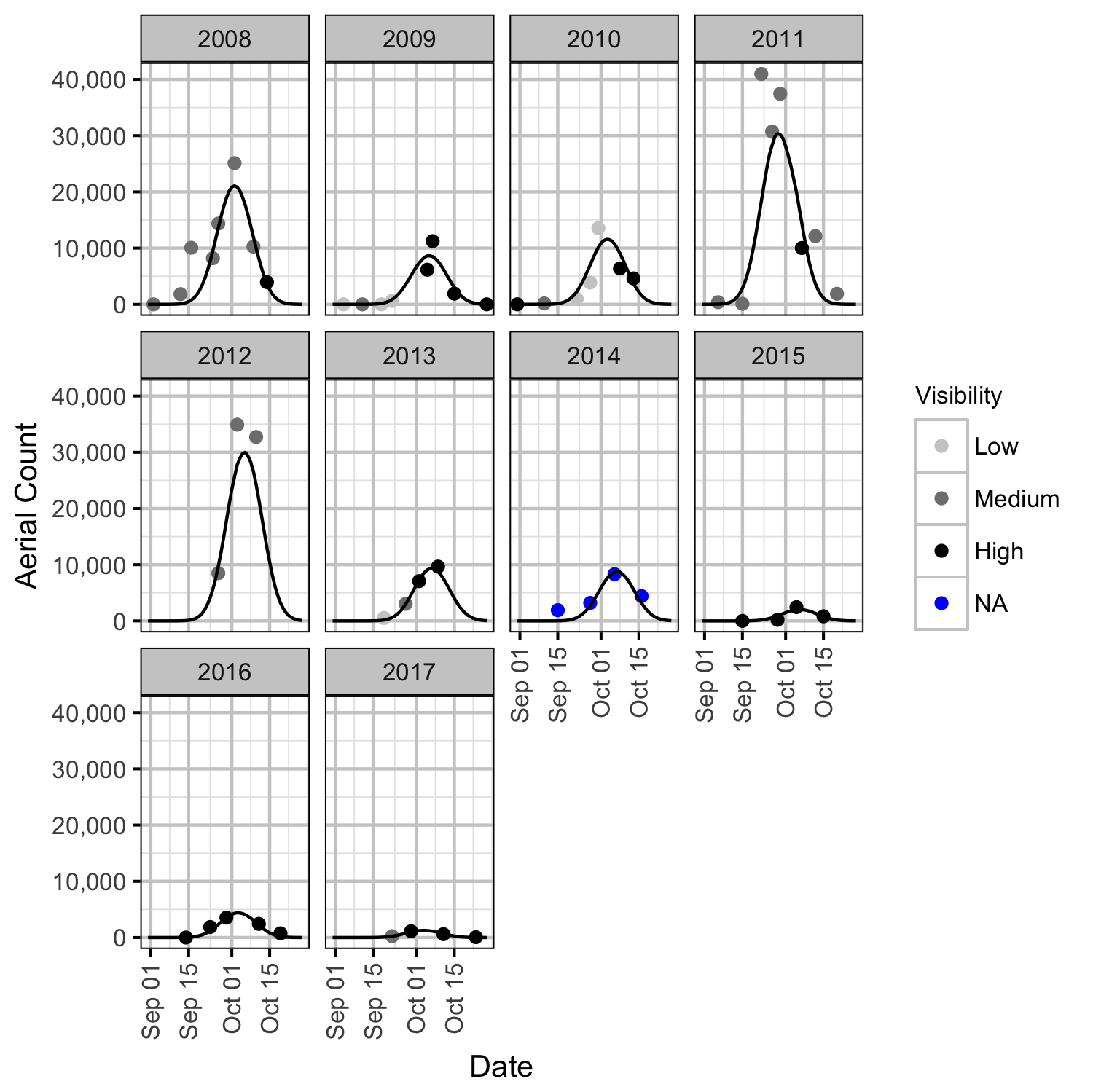
Abundance
Window
Acknowledgements
The organisations and individuals whose contributions have made this analysis report possible include:
- BC Hydro
- Guy Martel
- Alf Leake
- Okanagan National Alliance
- Michael Zimmer
- LGL Limited
- Elmar Plate
- MFLNRO
- Jeff Burrows
- Matt Neufeld
- Murray Pearson
- Marley Bassett
- Gerry Nellestijn
References
Acara, A. H. 1970. “The Meadow Creek Spawning Channel. Unpublished Report.” Victoria, BC: Fish; Wildlife Branch.
Bradford, Michael J, Josh Korman, and Paul S Higgins. 2005. “Using Confidence Intervals to Estimate the Response of Salmon Populations (Oncorhynchus Spp.) to Experimental Habitat Alterations.” Canadian Journal of Fisheries and Aquatic Sciences 62 (12): 2716–26. https://doi.org/10.1139/f05-179.
Hilborn, Ray, Brian G Bue, and Samuel Sharr. 1999. “Estimating Spawning Escapements from Periodic Counts: A Comparison of Methods.” Canadian Journal of Fisheries and Aquatic Sciences 56 (5): 888–96. https://doi.org/10.1139/f99-013.
Kery, Marc, and Michael Schaub. 2011. Bayesian Population Analysis Using WinBUGS : A Hierarchical Perspective. Boston: Academic Press. http://www.vogelwarte.ch/bpa.html.
McElreath, Richard. 2016. Statistical Rethinking: A Bayesian Course with Examples in R and Stan. Chapman & Hall/CRC Texts in Statistical Science Series 122. Boca Raton: CRC Press/Taylor & Francis Group.
Morbey, Y. E., and R. C. Ydenberg. 2003. “Timing Games in the Reproductive Phenology of Female Pacific Salmon (Oncorhynchus Spp.).” The American Naturalist 161 (2): 284–98. http://www.jstor.org/stable/10.1086/345785.
Plummer, Martyn. 2015. “JAGS Version 4.0.1 User Manual.” http://sourceforge.net/projects/mcmc-jags/files/Manuals/4.x/.
R Core Team. 2015. “R: A Language and Environment for Statistical Computing.” Vienna, Austria: R Foundation for Statistical Computing. http://www.R-project.org/.
———. 2016. “R: A Language and Environment for Statistical Computing.” Vienna, Austria: R Foundation for Statistical Computing. https://www.R-project.org/.
Su, Zhenming, Milo D. Adkison, and Benjamin W. Van Alen. 2001. “A Hierarchical Bayesian Model for Estimating Historical Salmon Escapement and Escapement Timing.” Canadian Journal of Fisheries and Aquatic Sciences 58 (8): 1648–62. https://doi.org/10.1139/cjfas-58-8-1648.
Wickham, Hadley. 2014. “Tidy Data.” Journal of Statistical Software 59 (10): 1–22. http://www.jstatsoft.org/v59/i10.