Lower Columbia River Rainbow Trout Spawning Analysis 2017
The suggested citation for this analytic report is:
Thorley, J.L., Muir, C.D. and Dalgarno, S. (2018) Lower Columbia River Rainbow Trout Spawning Analysis 2017. A Poisson Consulting Analysis Report. URL: https://www.poissonconsulting.ca/f/453582501.
Background
Each spring in the Lower Columbia River (LCR) below the Hugh L. Keenleyside Dam (HLK) and in the Lower Kootenay River (LKR) below the Brilliant Dam, thousands of Rainbow Trout spawn. Since 1992, BC Hydro has stabilized the spring discharge releases from HLK to protect Rainbow Trout redds from dewatering.
The primary goal of the current analysis to answer the following management questions:
Does the implementation of Rainbow Trout Spawning Protection Flows over the course of the monitoring period lead to an increase in the relative abundance of Rainbow Trout spawning in the LCR downstream of the HLK dam?
Does the implementation of RTSPF over the course of the monitoring period lead to an increase in the spatial distribution of locations (and associated habitat area) that Rainbow Trout use for spawning in the LCR downstream of HLK?
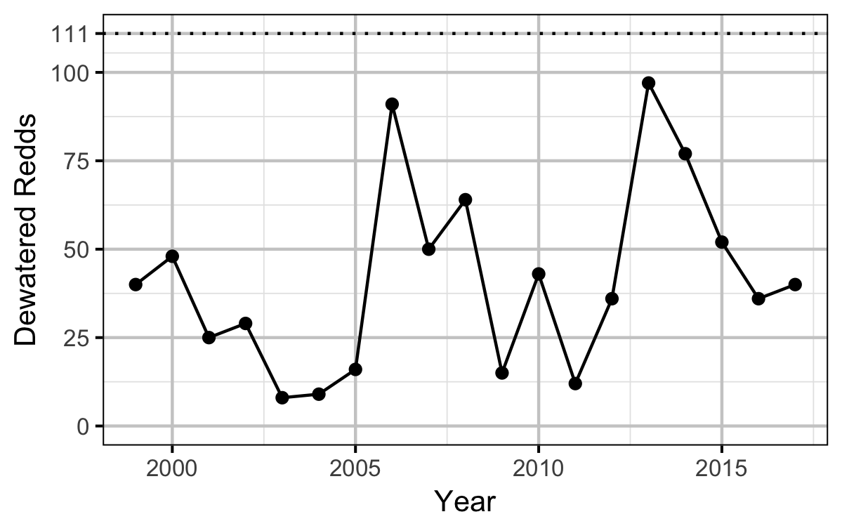
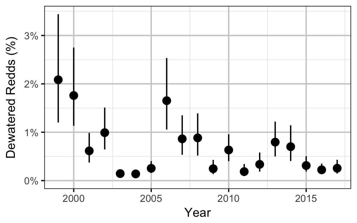
Does the implementation of RTSPF over the course of the monitoring period protect the majority of Rainbow Trout redds (as estimated from spawning timing) from being dewatered in the LCR downstream of HLK?
Data Preparation
The age-1 Rainbow Trout abundance data were provided by the Fish Population Indexing Program. The remaining fish data were collected by Mountain Water Research and imported to an SQLite database.
The study area was divided into three sections: the LCR above the LKR, the LKR and the LCR below the LKR. Redd and spawner counts upstream of Norns Creek Fan and downstream of Genelle were excluded from the section totals because they constitute less than 0.1% of the total count and were not surveyed in all years. The redd and spawner counts for the Right Upstream Bank above Robson Bridge were also excluded as they appear to be primarily driven by viewing conditions (and constitute less than 2.5% of the total). Viewing conditions were classified as Good or Poor. If information on the viewing conditions was not available a decline in the redd count of more than one third of the cumulative maximum count for a particular section was assumed to be caused by poor viewing conditions.
The data were prepared for analysis using R version 3.4.4 (R Core Team 2017).
Statistical Analysis
Model parameters were estimated using Bayesian methods. The Bayesian estimates were produced using JAGS (Plummer 2015) and Stan (Carpenter et al. 2017). For additional information on Bayesian modelling in the BUGS language, of which JAGS uses a dialect, the reader is referred to Kery and Schaub (2011). For additional information on Bayesian modelling in the Stan language the reader is referred to Stan Development Team (2017).
Unless indicated otherwise, the Bayesian analyses used uninformative uniform or normal prior distributions (Kery and Schaub 2011, 36). The posterior distributions were estimated from 1,500 Markov Chain Monte Carlo (MCMC) samples thinned from the second halves of three chains (Kery and Schaub 2011, 38–40). Model convergence was confirmed by ensuring that \(\hat{R} < 1.1\) (Kery and Schaub 2011, 40) for each of the monitored parameters (Kery and Schaub 2011, 61).
The parameters are summarised in terms of the point estimate, standard deviation (sd), the z-score, lower and upper 95% credible limits (CLs) and the p-value (Kery and Schaub 2011, 37, 42). A p-value of 0.05 indicates that the lower or upper 95% CL is 0. The estimate is the median (50th percentile) of the MCMC samples, the z-score is \(\mathrm{mean}/\mathrm{sd}\) and the 95% CLs are the 2.5th and 97.5th percentiles.
The results are displayed graphically by plotting the modeled relationships between particular variables and the response(s) with the remaining variables held constant. In general, continuous and discrete fixed variables are held constant at their mean and first level values, respectively, while random variables are held constant at their typical values (expected values of the underlying hyperdistributions) (Kery and Schaub 2011, 77–82). When informative the influence of particular variables is expressed in terms of the effect size (i.e., percent change in the response variable) with 95% confidence/credible intervals (CIs, Bradford, Korman, and Higgins 2005).
The analyses were implemented using R version 3.4.4
(R Core Team 2017) and the jmbr and smbr packages.
Model Descriptions
Norns Creek
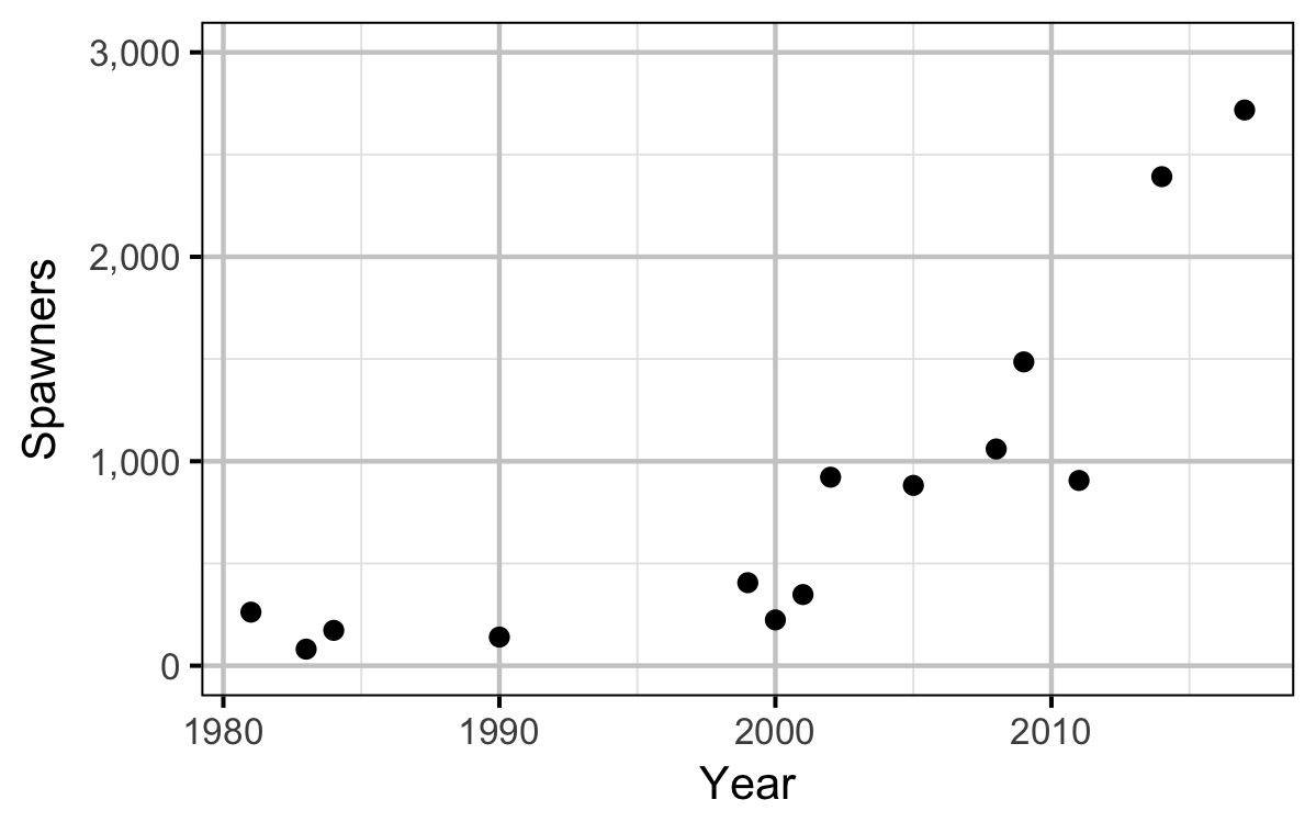
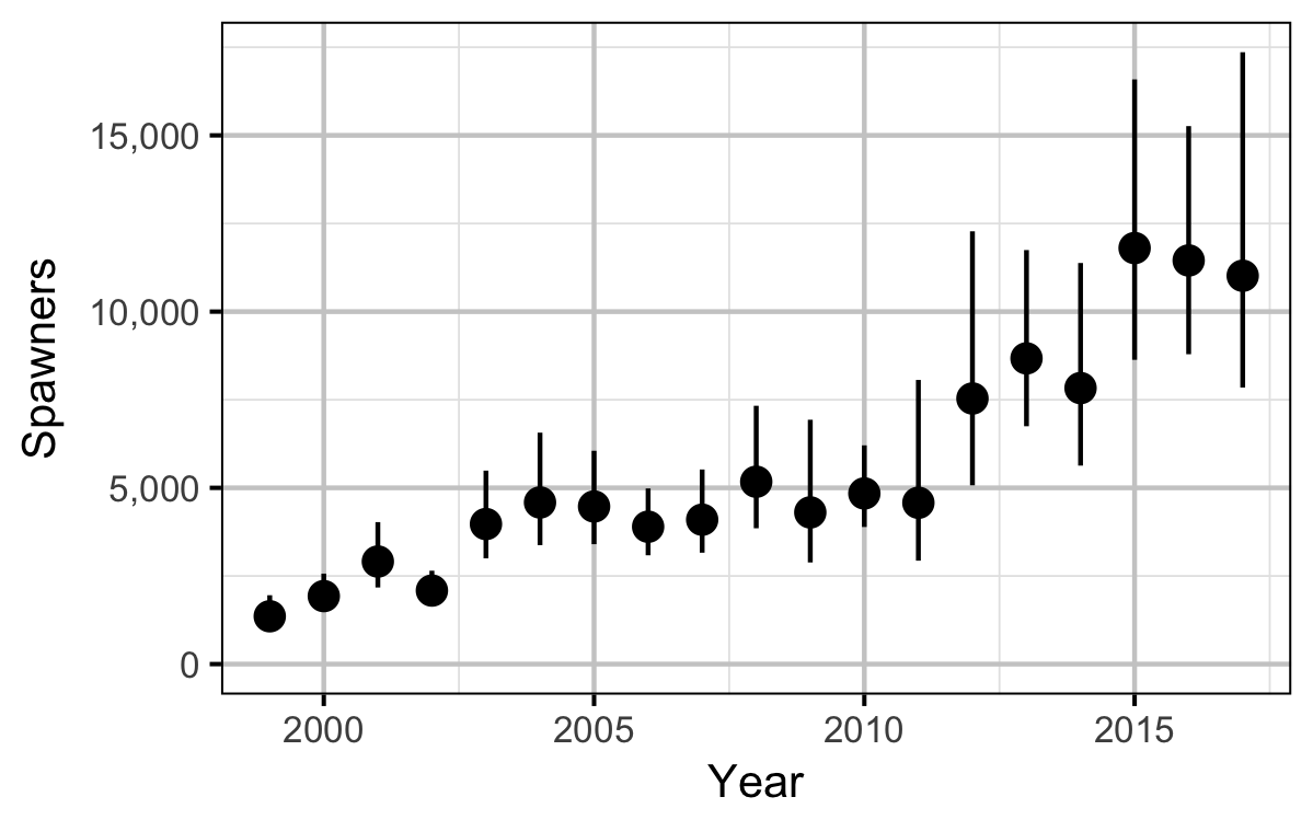
Following Thorley and Baxter (2012), the peak spawner counts from 1999 were multiplied by an expansion factor of two to get the estimated spawner abundance and combined with historical spawner abundance estimates.
Distribution
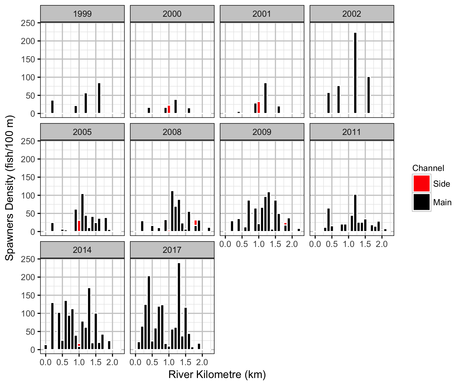
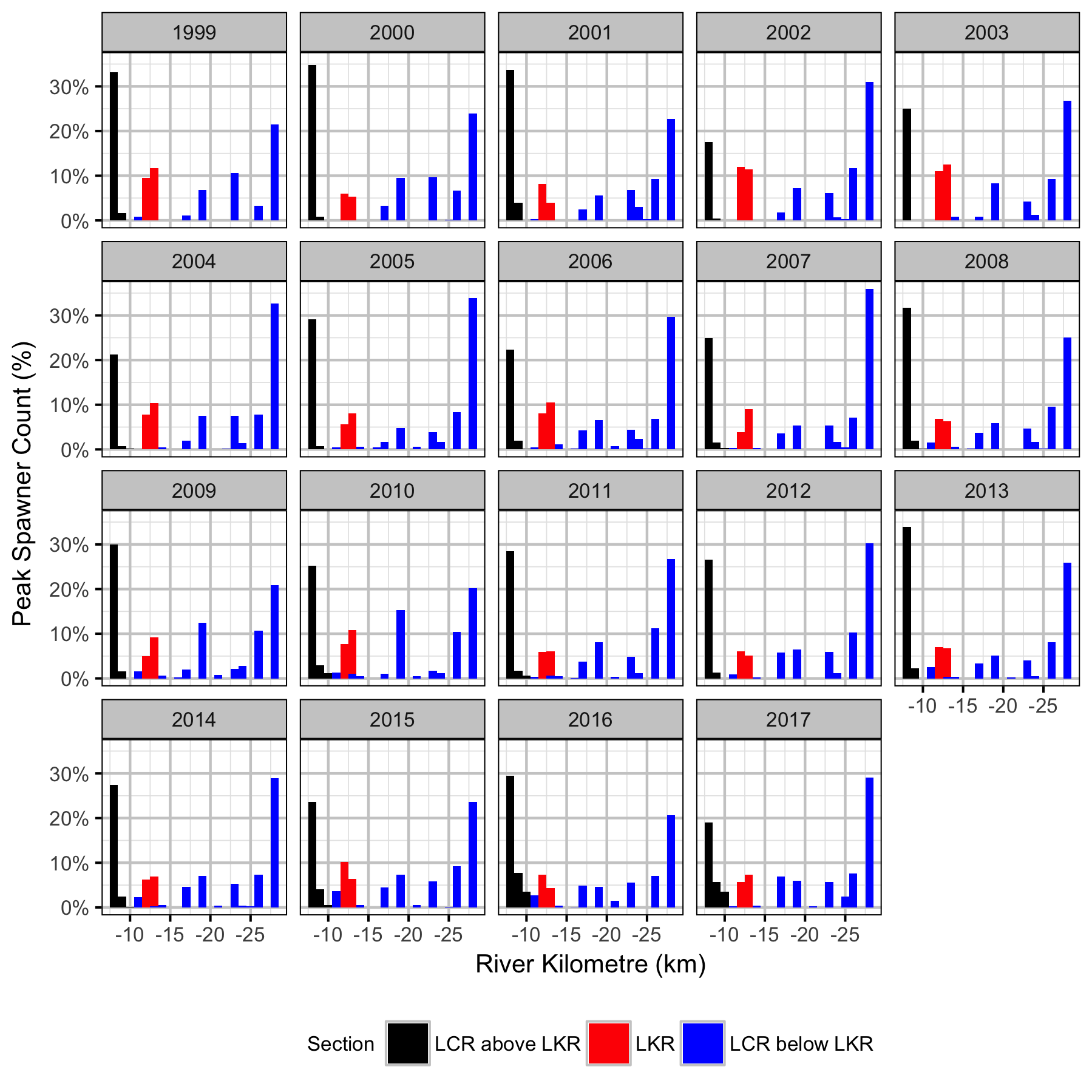
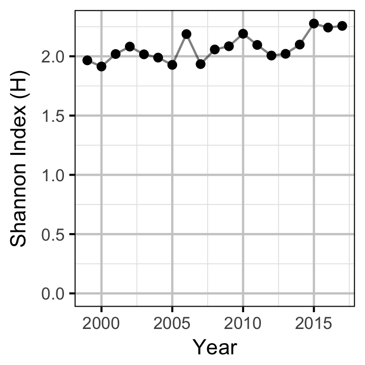
The proportion of fish were plotted by river km and year for the day of the peak spawner count to visualize the distribution of spawning. The Shannon Index \(H\) was calculated for each year where \[ H = - \sum{p_i log(p_i)}\] and \(p_i\) is the proportion of the spawners at the \(i\)th site with a positive count.
Area-Under-The-Curve
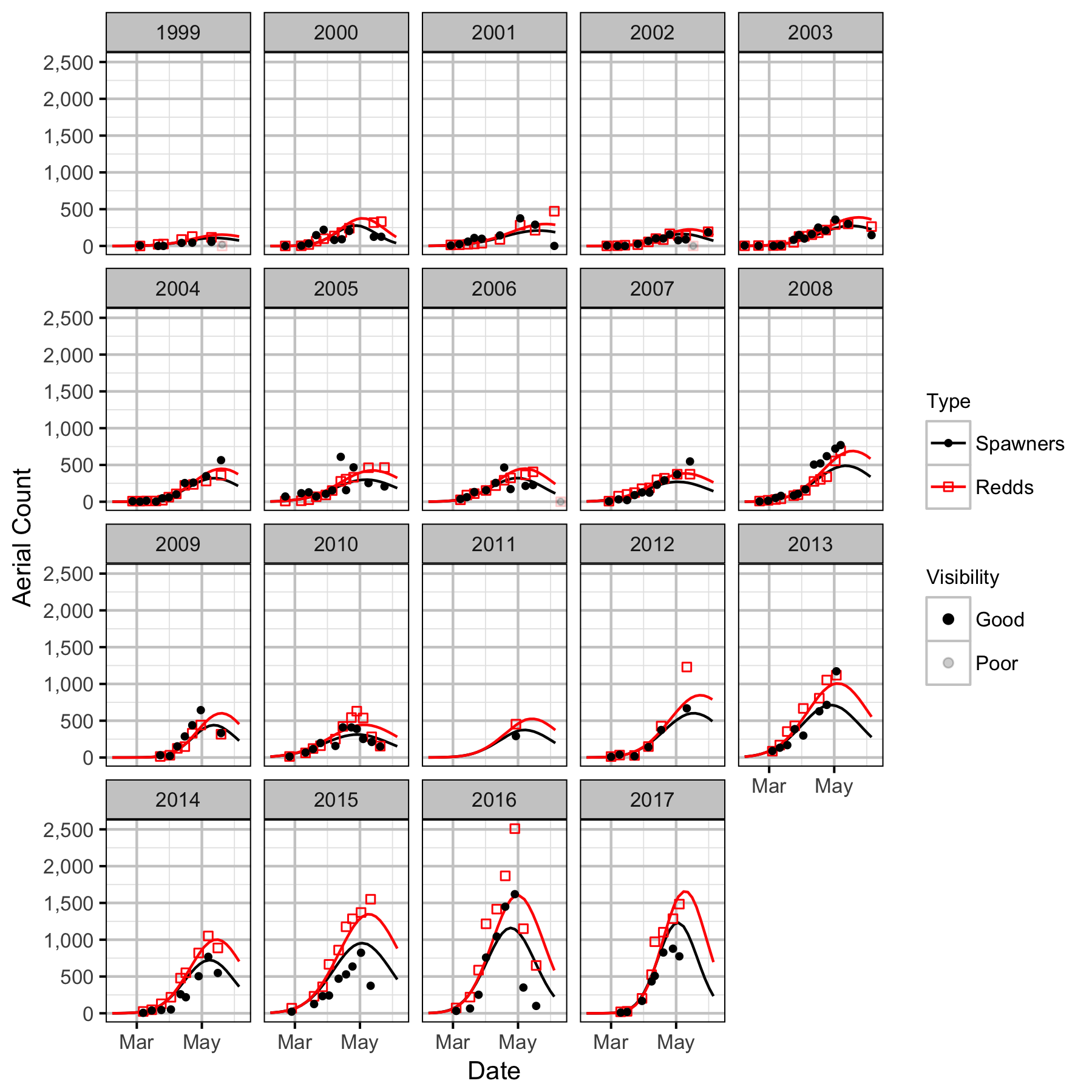
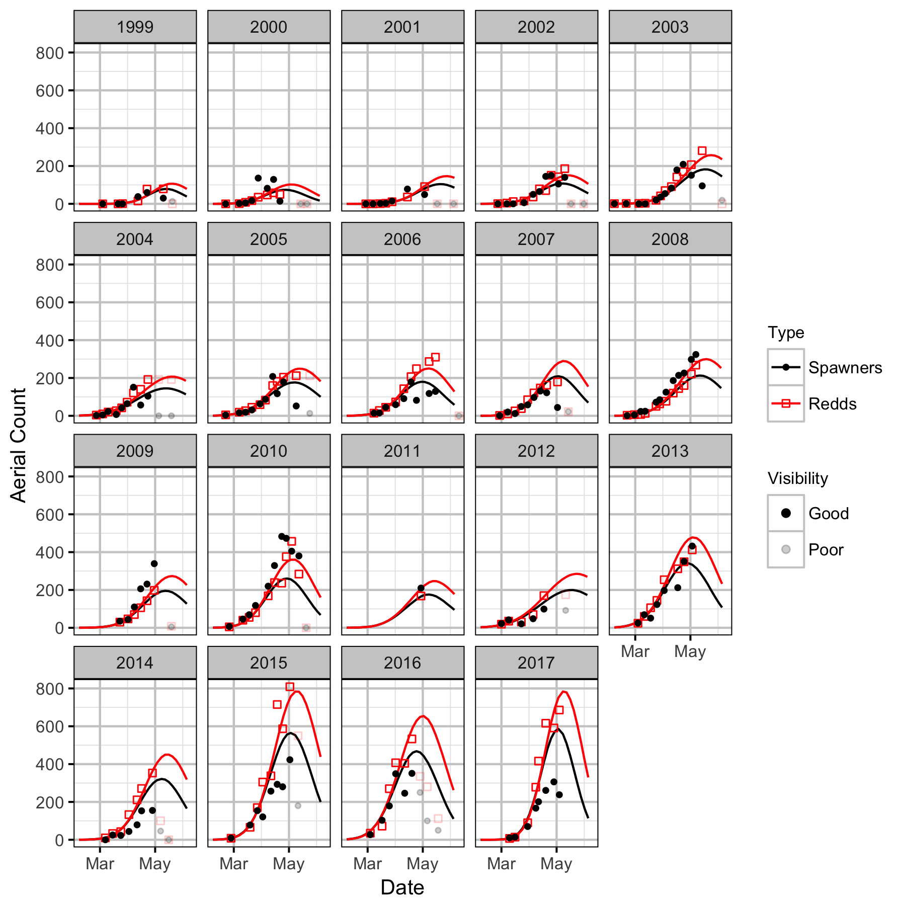
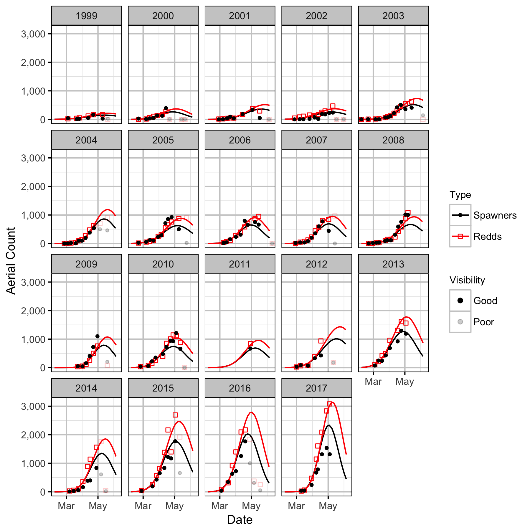
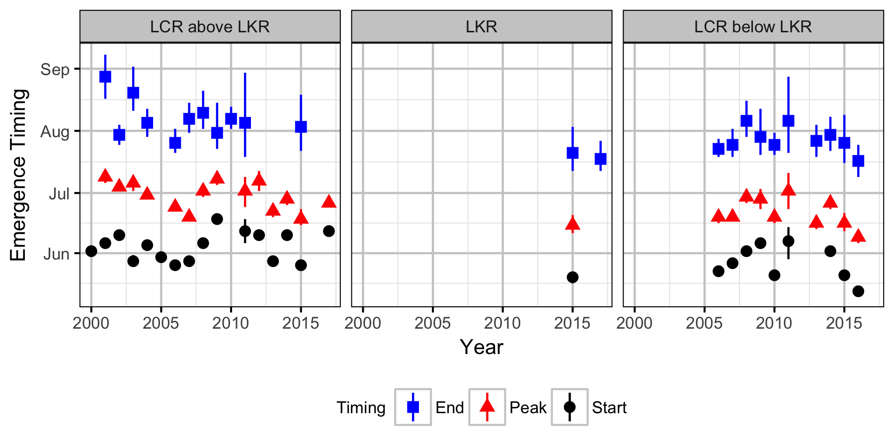
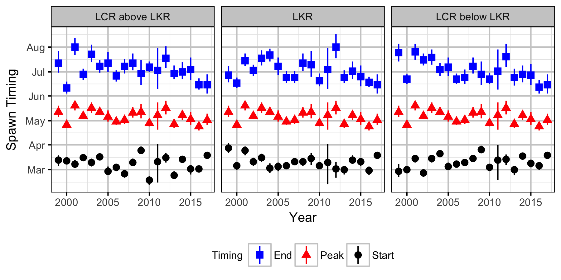
The spawner abundance and spawn timings were estimated from the aerial fish and redd counts for the three sections using an Area-Under-The-Curve (AUC) model.
Key assumptions of the AUC model include:
- Spawner abundance varies by river section.
- Spawner abundance varies randomly by year and section within year.
- Spawner observer efficiency is between 0.8 and 1.0.
- Number of redds per spawner is between 1 and 2.
- Spawner residence time is between 14 and 21 days as determined in a previous year’s analysis.
- Redd residence time is between 30 and 40 days.
- Spawner arrival and departure times are normally distributed.
- Spawner arrival duration (SD of normal distribution) varies randomly by section within year.
- Peak spawner arrival timing varies randomly by year.
- The residual variations in the spawner and redd counts are described by separate Negative Binomial distributions.
Preliminary analysis of skew normal and sine arrival and departure functions did not improve the fit of the model.
Stock-Recruitment
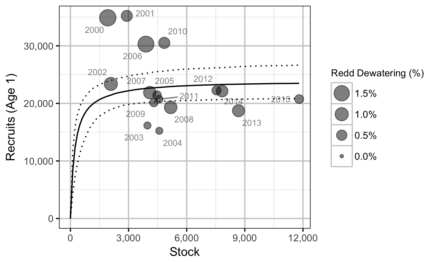
The relationship between the number of spawners and the resultant number of age-1 fish was estimated using a Beverton-Holt stock-recruitment model (Walters and Martell 2004):
\[ R = \frac{\alpha \cdot S}{1 + \beta \cdot S} \quad,\]
where \(S\) is the spawners (stock), \(R\) is the recruits, \(\alpha\) is the recruits per spawner at low density and \(\beta\) determines the density-dependence.
Key assumptions of the stock-recruitment model include:
- The recruits per spawner at low density (\(\alpha\)) is normally distributed with a mean of 90 and a SD of 50.
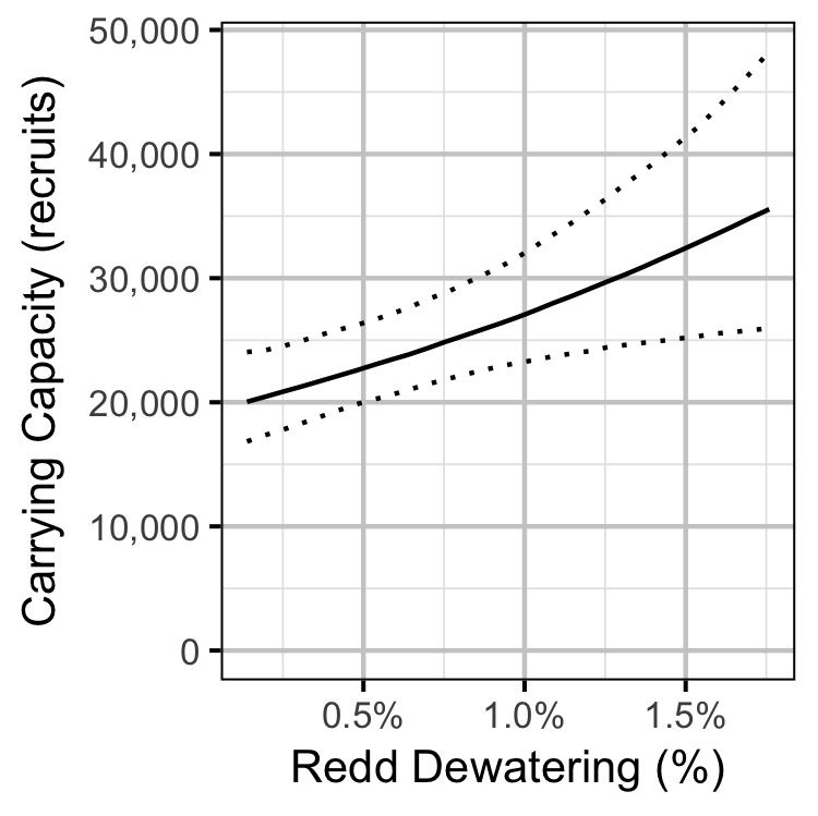
- The recruits per spawner varies with the percent of redds dewatered.
- The residual variation in the number of recruits is log-normally distributed.
The mean of 90 for \(\alpha\) was based on an average of 2,900 eggs per female spawner, a 50:50 sex ratio, 50% egg survival, 50% post-emergence fall survival, 50% overwintering survival and 50% summer survival.
The carrying capacity is \(\alpha / \beta\).
Model Templates
Area-Under-The-Curve
data {
  int<lower=0> nObs;
  int<lower=0> nSection;
  int<lower=0> nYear;

  int Year[nObs];
  int Section[nObs];
  real Doy[nObs];
  int Spawners[nObs];
  int Redds[nObs];
parameters {
  vector<lower=5,upper=10>[nSection] bSpawnerAbundanceSection;

  real<lower=0,upper=2> sSpawnerAbundanceYear;
  vector[nYear] bSpawnerAbundanceYear;
  real<lower=0,upper=2> sSpawnerAbundanceSectionYear;
  vector[nSection * nYear] bSpawnerAbundanceSectionYear;

  real<lower=0.8,upper=1.0> bSpawnerObserverEfficiency;
  real<lower=0.0,upper=2.0> bReddObserverEfficiency;

  real<lower=1, upper=2> bReddPerSpawner;

  real<lower=14, upper=21> bSpawnerResidenceTime;
  real<lower=30, upper=40> bReddResidenceTime;

  real<lower=100, upper=150> bPeakSpawnerArrivalTiming;

  real<lower=0,upper=21> sPeakSpawnerArrivalTimingYear;
  vector[nYear] bPeakSpawnerArrivalTimingYear;

  real<lower=log(10), upper=log(50)> bSpawnerArrivalDuration;

  real<lower=0,upper=2> sSpawnerArrivalDurationSectionYear;
  vector[nSection * nYear] bSpawnerArrivalDurationSectionYear;

  real<lower=0, upper=2> bDispersionRedds;
  real<lower=0, upper=2> bDispersionSpawners;
model {
  vector[nObs] eSpawnerAbundance;
  vector[nObs] ePeakSpawnerArrivalTiming;
  vector[nObs] eSpawnerArrivalDuration;

  vector[nObs] eRedds;
  vector[nObs] eSpawners;

  bSpawnerAbundanceYear ~ normal(0, sSpawnerAbundanceYear);
  bSpawnerAbundanceSectionYear ~ normal(0, sSpawnerAbundanceSectionYear);

  bPeakSpawnerArrivalTimingYear ~ normal(0, sPeakSpawnerArrivalTimingYear);
  bSpawnerArrivalDurationSectionYear ~ normal(0, sSpawnerArrivalDurationSectionYear);

  for (i in 1:nObs) {
    eSpawnerAbundance[i] = exp(bSpawnerAbundanceSection[Section[i]] + bSpawnerAbundanceYear[Year[i]] + bSpawnerAbundanceSectionYear[((Section[i] - 1) * Year[i]) + Year[i]]);

    ePeakSpawnerArrivalTiming[i] = bPeakSpawnerArrivalTiming + bPeakSpawnerArrivalTimingYear[Year[i]];

    eSpawnerArrivalDuration[i] = exp(bSpawnerArrivalDuration + bSpawnerArrivalDurationSectionYear[((Section[i] - 1) * Year[i]) + Year[i]]);

    eRedds[i] = eSpawnerAbundance[i] * bReddPerSpawner * bReddObserverEfficiency * (normal_cdf(Doy[i], ePeakSpawnerArrivalTiming[i], eSpawnerArrivalDuration[i]) - normal_cdf(Doy[i], ePeakSpawnerArrivalTiming[i] + bReddResidenceTime, eSpawnerArrivalDuration[i]));

    eSpawners[i] = eSpawnerAbundance[i] * bSpawnerObserverEfficiency * (normal_cdf(Doy[i], ePeakSpawnerArrivalTiming[i], eSpawnerArrivalDuration[i]) - normal_cdf(Doy[i], ePeakSpawnerArrivalTiming[i] + bSpawnerResidenceTime, eSpawnerArrivalDuration[i]));
  }
  Redds ~ neg_binomial_2(eRedds, 1/bDispersionRedds);
  Spawners ~ neg_binomial_2(eSpawners, 1/bDispersionSpawners);
..
Template 1. AUC model.
Stock-Recruitment
model {

  bAlpha ~ dnorm(90, 50^-2) T(1,)
  bAlphaDewatered ~ dnorm(0, 2^-2)
  bBeta ~ dnorm(-5, 5^-2)
  sRecruits ~ dunif(0, 2)

  for(i in 1:length(Stock)) {
    log(eAlpha[i]) <- log(bAlpha) + bAlphaDewatered * Dewatered[i]
    log(eBeta[i]) <- bBeta
    eRecruits[i] <- eAlpha[i] * Stock[i] / (1 + eBeta[i] * Stock[i])
    Recruits[i] ~ dlnorm(log(eRecruits[i]), sRecruits^-2)
  }
..
Template 2.
Results
Tables
Area-Under-The-Curve
Table 1. Parameter descriptions.
| Parameter | Description |
|---|---|
bDispersionRedds |
Clustering parameter for Redds |
bDispersionSpawners |
Clustering parameter for Spawner |
bPeakSpawnerArrivalTiming |
Intercept for ePeakSpawnerArrivalTiming |
bPeakSpawnerArrivalTimingYear[i] |
Effect of ith Year on
bPeakSpawnerArrivalTiming |
bReddObserverEfficiency |
Redd observer efficiency |
bReddPerSpawner |
Number of redds per spawner |
bReddResidenceTime |
Redd residence time (days) |
bSpawnerAbundanceSection[i] |
Intercept for log(eSpawnerAbundance) by
Section |
bSpawnerAbundanceSectionYear[i] |
Effect of Section by Year on
bSpawnerAbundanceSection |
bSpawnerAbundanceYear[i] |
Effect of ith Year on
bSpawnerAbundanceSection |
bSpawnerArrivalDuration[i] |
Intercept for
log(eSpawnerArrivalDuration) |
bSpawnerArrivalDurationSectionYear[i] |
Effect of Section by Year on
bSpawnerArrivalDuration |
bSpawnerObsEfficiency |
Spawner observer efficiency |
bSpawnerResidenceTime |
Spawner residence time (days) |
Doy[i] |
Day of the year of ith count |
ePeakSpawnerArrivalTiming[i] |
Expected Doy of peak spawner arrival for
ith count |
eSpawnerAbundance[i] |
Expected spawner abundance for ith
count |
eSpawnerArrivalDuration[i] |
Expected SD of spawner arrival timing for
ith count |
Redds[i] |
Observed number of redds on ith count |
Section[i] |
Section of ith count |
Spawners[i] |
Observed number of fish on ith count |
sPeakSpawnerArrivalTimingYear |
SD of bPeakSpawnerArrivalTimingYear |
sSpawnerAbundanceSectionYear |
SD of bSpawnerAbundanceSectionYear |
sSpawnerAbundanceYear |
SD of bSpawnerAbundanceYear |
sSpawnerArrivalDurationSectionYear |
SD of bSpawnerArrivalDurationSectionYear |
Year[i] |
Year of ith count |
Table 2. Model coefficients.
| term | estimate | sd | zscore | lower | upper | pvalue |
|---|---|---|---|---|---|---|
| bDispersionRedds | 0.0639992 | 0.0063876 | 10.035942 | 0.0523664 | 0.0772205 | 7e-04 |
| bDispersionSpawners | 0.3578947 | 0.0291376 | 12.329979 | 0.3075142 | 0.4202275 | 7e-04 |
| bPeakSpawnerArrivalTiming | 117.7704101 | 2.5624245 | 45.930831 | 112.3787075 | 122.4990774 | 7e-04 |
| bReddObserverEfficiency | 0.5575340 | 0.1230811 | 4.650286 | 0.3807214 | 0.8212783 | 7e-04 |
| bReddPerSpawner | 1.4072730 | 0.2875174 | 4.984488 | 1.0128960 | 1.9581605 | 7e-04 |
| bReddResidenceTime | 32.1717041 | 2.1077375 | 15.489881 | 30.1153488 | 37.9404678 | 7e-04 |
| bSpawnerAbundanceSection[1] | 7.2931052 | 0.1743077 | 41.901327 | 6.9828132 | 7.6643588 | 7e-04 |
| bSpawnerAbundanceSection[2] | 6.5980752 | 0.1739736 | 37.977992 | 6.2926927 | 6.9713950 | 7e-04 |
| bSpawnerAbundanceSection[3] | 7.8369781 | 0.1732353 | 45.312943 | 7.5296782 | 8.2181848 | 7e-04 |
| bSpawnerArrivalDuration | 3.1770508 | 0.0397765 | 79.882724 | 3.0986767 | 3.2587875 | 7e-04 |
| bSpawnerObserverEfficiency | 0.9044389 | 0.0582377 | 15.507867 | 0.8047635 | 0.9956511 | 7e-04 |
| bSpawnerResidenceTime | 19.7695258 | 1.3364750 | 14.511193 | 15.9795858 | 20.9459947 | 7e-04 |
| sPeakSpawnerArrivalTimingYear | 8.6441834 | 1.9251474 | 4.661460 | 6.0590174 | 13.4810353 | 7e-04 |
| sSpawnerAbundanceSectionYear | 0.1489069 | 0.0334226 | 4.560084 | 0.0956515 | 0.2281738 | 7e-04 |
| sSpawnerAbundanceYear | 0.6187568 | 0.1197512 | 5.324793 | 0.4516900 | 0.9066212 | 7e-04 |
| sSpawnerArrivalDurationSectionYear | 0.1875548 | 0.0295313 | 6.442084 | 0.1373939 | 0.2555155 | 7e-04 |
Table 3. Model summary.
| n | K | nchains | niters | nthin | ess | rhat | converged |
|---|---|---|---|---|---|---|---|
| 472 | 16 | 3 | 500 | 1 | 225 | 1.02 | TRUE |
Stock-Recruitment
Table 4. Parameter descriptions.
| Parameter | Description |
|---|---|
bAlpha |
Intercept for eAlpha |
bAlphaDewatered |
Effect of Dewatered on log(bAlpha) |
bBeta |
Intercept for log(eBeta) |
Dewatered[i] |
Proportional redd dewatering in ith spawn year |
eAlpha |
Expected number of recruits at low density |
eBeta |
Expected density-dependence |
eRecruits[i] |
Expected Recruits |
Recruits[i] |
Number of age-1 recruits from ith spawn year |
sRecruits |
SD of residual variation in Recruits |
Stock[i] |
Number of spawners in ith spawn year |
Table 5. Model coefficients.
| term | estimate | sd | zscore | lower | upper | pvalue |
|---|---|---|---|---|---|---|
| bAlpha | 107.8448855 | 40.6515663 | 2.725891 | 42.1359752 | 197.4604192 | 0.0007 |
| bAlphaDewatered | 0.1758749 | 0.0605724 | 2.900793 | 0.0522337 | 0.2928220 | 0.0107 |
| bBeta | -5.4023315 | 0.4307361 | -12.661583 | -6.3983370 | -4.7680197 | 0.0007 |
| sRecruits | 0.2182466 | 0.0495995 | 4.551917 | 0.1530152 | 0.3444041 | 0.0007 |
Table 6. Model summary.
| n | K | nchains | niters | nthin | ess | rhat | converged |
|---|---|---|---|---|---|---|---|
| 16 | 4 | 3 | 500 | 1000 | 1020 | 1 | TRUE |
Figures
Distribution
Stock-Recruitment
Discharge
Recommendations
- Redd viewing conditions should be updated to take into account the fact that redds are static and may not be visible when water levels rise even if viewing conditions are good.
Acknowledgements
The organisations and individuals whose contributions have made this analysis report possible include:
- BC Hydro
- Darin Nishi
- Margo Dennis
- Guy Martel
- Philip Bradshaw
- James Baxter
- Mountain Water Research
- Jeremy Baxter
- Poisson Consulting
- Robyn Irvine
- Dam Helicopters
- Duncan Wassick
- Highland Helicopters
- Phil Hocking
- Mark Homis
- Golder Associates
- Dustin Ford
- Demitria Burgoon
- David Roscoe
- Additional Support
- Clint Tarala
- Crystal Lawrence
- Gary Pavan
- Gerry Nellestijn
- Jay Bowers
References
Bradford, Michael J, Josh Korman, and Paul S Higgins. 2005. “Using Confidence Intervals to Estimate the Response of Salmon Populations (Oncorhynchus Spp.) to Experimental Habitat Alterations.” Canadian Journal of Fisheries and Aquatic Sciences 62 (12): 2716–26. https://doi.org/10.1139/f05-179.
Carpenter, Bob, Andrew Gelman, Matthew D. Hoffman, Daniel Lee, Ben Goodrich, Michael Betancourt, Marcus Brubaker, Jiqiang Guo, Peter Li, and Allen Riddell. 2017. “Stan : A Probabilistic Programming Language.” Journal of Statistical Software 76 (1). https://doi.org/10.18637/jss.v076.i01.
Kery, Marc, and Michael Schaub. 2011. Bayesian Population Analysis Using WinBUGS : A Hierarchical Perspective. Boston: Academic Press. http://www.vogelwarte.ch/bpa.html.
Plummer, Martyn. 2015. “JAGS Version 4.0.1 User Manual.” http://sourceforge.net/projects/mcmc-jags/files/Manuals/4.x/.
R Core Team. 2017. “R: A Language and Environment for Statistical Computing.” Vienna, Austria: R Foundation for Statistical Computing. https://www.R-project.org/.
Stan Development Team. 2017. “Stan Modeling Language Users Guide and Reference Manual.” http://mc-stan.org.
Thorley, J. L., and J. T. A. Baxter. 2012. “Lower Columbia River Rainbow Trout Spawning Assessment: Year 4 (2011 Study Period).” A Mountain Waters Research Report. Castlegar, BC: BC Hydro. http://www.bchydro.com/etc/medialib/internet/documents/planning_regulatory/wup/southern_interior/2012q1/clbmon-46_yr4_2012-02-08.Par.0001.File.CLBMON-46-Yr4-2012-02-08.pdf.
Walters, Carl J., and Steven J. D. Martell. 2004. Fisheries Ecology and Management. Princeton, N.J: Princeton University Press.