Lower Columbia River Fish Population Indexing 2020
The suggested citation for this analytic report is:
Thorley, J.L. & Hussein, N. (2021) Lower Columbia River Fish Population Indexing 2020. A Poisson Consulting Analytic Appendix. URL: https://www.poissonconsulting.ca/f/392669554.
Background
In the mid 1990s BC Hydro began operating Hugh L. Keenleyside (HLK) Dam to reduce dewatering of Mountain Whitefish and Rainbow Trout eggs.
The primary goal of the Lower Columbia River Fish Population Indexing program is to answer two key management questions:
What are the abundance, growth rate, survival rate, body condition, age distribution, and spatial distribution of subadult and adult Whitefish, Rainbow Trout, and Walleye in the Lower Columbia River?
What is the effect of inter-annual variability in the Whitefish and Rainbow Trout flow regimes on the abundance, growth rate, survival rate, body condition, and spatial distribution of subadult and adult Whitefish, Rainbow Trout, and Walleye in the Lower Columbia River?
The inter-annual variability in the Whitefish and Rainbow Trout flow regimes was quantified in terms of the percent egg dewatering as greater flow variability is associated with more egg stranding.
Methods
Data Preparation
The fish indexing data were provided by Okanagan Nation Alliance and Golder Associates in the form of an Access database. The discharge and temperature data were obtained from the Columbia Basin Hydrological Database maintained by Poisson Consulting. The Rainbow Trout egg dewatering estimates were provided by CLBMON-46 (Irvine, Baxter, and Thorley 2015) and the Mountain Whitefish egg stranding estimates by Golder Associates (2013).
Discharge
Missing hourly discharge values for Hugh-Keenleyside Dam (HLK), Brilliant Dam (BRD) and Birchbank (BIR) were estimated by first leading the BIR values by 2 hours to account for the lag. Values missing at just one of the dams were then estimated assuming \(HLK + BRD = BIR\). Negative values were set to be zero. Next, missing values spanning \(\leq\) 28 days were estimated at HLK and BRD based on linear interpolation. Finally any remaining missing values at BIR were set to be \(HLK + BRD\).
The data were prepared for analysis using R version 4.1.1 (R Core Team 2018).
Data Analysis
Model parameters were estimated using hierarchical Bayesian methods. The parameters were produced using JAGS (Plummer 2015) and STAN (Carpenter et al. 2017). For additional information on Bayesian estimation the reader is referred to McElreath (2016).
The one exception is the length-at-age estimates which were produced using the mixdist R package (P. Macdonald 2012) which implements Maximum Likelihood with Expectation Maximization.
Unless stated otherwise, the Bayesian analyses used weakly informative normal and half-normal prior distributions (Gelman, Simpson, and Betancourt 2017). The posterior distributions were estimated from 1500 Markov Chain Monte Carlo (MCMC) samples thinned from the second halves of 3 chains (Kery and Schaub 2011, 38–40). Model convergence was confirmed by ensuring that the potential scale reduction factor \(\hat{R} \leq 1.05\) (Kery and Schaub 2011, 40) and the effective sample size (Brooks et al. 2011) \(\textrm{ESS} \geq 150\) for each of the monitored parameters (Kery and Schaub 2011, 61).
The parameters are summarised in terms of the point estimate, lower and upper 95% credible limits (CLs) and the surprisal s-value (Greenland 2019). The estimate is the median (50th percentile) of the MCMC samples while the 95% CLs are the 2.5th and 97.5th percentiles. The s-value can be considered a test of directionality. More specifically it indicates how surprising (in bits) it would be to discover that the true value of the parameter is in the opposite direction to the estimate. An s-value (Chow and Greenland 2019) is the Shannon transform (-log to base 2) of the corresponding p-value (Kery and Schaub 2011; Greenland and Poole 2013). A surprisal value of 4.3 bits, which is equivalent to a p-value of 0.05 indicates that the surprise would be equivalent to throwing 4.3 heads in a row. The condition that non-essential explanatory variables have s-values \(\geq\) 4.3 bits provides a useful model selection heuristic (Kery and Schaub 2011).
Model adequacy was assessed via posterior predictive checks (Kery and Schaub 2011). More specifically, the number of zeros and the first four central moments (mean, variance, skewness and kurtosis) for the deviance residuals were compared to the expected values by simulating new residuals. In this context the s-value indicates how surprising each metric is given the estimated posterior probability distribution for the residual variation.
Where computationally practical, the sensitivity of the parameters to the choice of prior distributions was evaluated by increasing the standard deviations of all normal, half-normal and log-normal priors by an order of magnitude and then using \(\hat{R}\) to test whether the samples where drawn from the same posterior distribution (Thorley and Andrusak 2017).
The results are displayed graphically by plotting the modeled relationships between particular variables and the response(s) with the remaining variables held constant. In general, continuous and discrete fixed variables are held constant at their mean and first level values, respectively, while random variables are held constant at their typical values (expected values of the underlying hyperdistributions) (Kery and Schaub 2011, 77–82). When informative the influence of particular variables is expressed in terms of the effect size (i.e., percent or n-fold change in the response variable) with 95% credible intervals (CIs, Bradford, Korman, and Higgins 2005).
The analyses were implemented using R version 4.1.1
(R Core Team 2020) and the
mbr family of packages.
Model Descriptions
Condition
The expected weight of fish of a given length were estimated from the data using an allometric mass-length model (He et al. 2008).
\[W = \alpha L^{\beta}\]
Key assumptions of the condition model include:
- The expected weight is allowed to vary with length and date.
- The expected weight is allowed to vary randomly with year.
- The relationship between weight and length is allowed to vary with date.
- The relationship between weight and length is allowed to vary randomly with year.
- The residual variation in weight is log-normally distributed.
Only previously untagged fish were included in models to avoid potential effects of tagging on body condition. Preliminary analyses indicated that the annual variation in weight was not correlated with the annual variation in the relationship between weight and length.
Growth
Annual growth of fish were estimated from the inter-annual recaptures using the Fabens method (Fabens 1965) for estimating the von Bertalanffy growth curve (von Bertalanffy 1938). This curve is based on the premise that:
\[ \frac{\text{d}L}{\text{d}t} = k (L_{\infty} - L)\]
where \(L\) is the length of the individual, \(k\) is the growth coefficient and \(L_{\infty}\) is the maximum length.
Integrating the above equation gives:
\[ L_t = L_{\infty} (1 - e^{-k(t - t_0)})\]
where \(L_t\) is the length at time \(t\) and \(t_0\) is the time at which the individual would have had zero length.
The Fabens form allows
\[ L_r = L_c + (L_{\infty} - L_c) (1 - e^{-kT})\]
where \(L_r\) is the length at recapture, \(L_c\) is the length at capture and \(T\) is the time between capture and recapture.
Key assumptions of the growth model include:
- The mean maximum length \(L_{\infty}\) is constant.
- The growth coefficient \(k\) is allowed to vary randomly with year.
- The residual variation in growth is normally distributed.
The growth model was only fitted to Walleye with a fork length at release less than 450 mm.
Movement
The extent to which sites are closed, i.e., fish remain at the same site between sessions, was evaluated with a logistic ANCOVA (Kery 2010). The model estimates the probability that intra-annual recaptures were caught at the same site versus a different one. Key assumptions of the site fidelity model include:
- The expected site fidelity is allowed to vary with fish length.
- Observed site fidelity is Bernoulli distributed.
Length as a second-order polynomial was not found to be a significant predictor for site fidelity.
The estimated probability of being caught at the same site versus a different site was then converted into the site fidelity by assuming that those fish which were recaught at a different site represented just 32 % of those that left the site. The correction factor corresponds to the proportion of the river bank that belongs to index sites.
Length-At-Age
The expected length-at-age of Mountain Whitefish and Rainbow Trout were estimated from annual length-frequency distributions using a finite mixture distribution model (P. D. M. Macdonald and Pitcher 1979)
There were assumed to be three distinguishable normally-distributed age-classes for Mountain Whitefish (Age-0, Age-1, Age-2 and Age-3+) two for Rainbow Trout (Age-0, Age-1, Age-2+). Initially the model was fitted to the data from all years combined. The model was then fitted to the data for each year separately with the initial values set to be the estimates from the combined values. The only constraints were that the standard deviations of the MW age-classes were identical in the combined analysis and fixed at the initial values in the individual years.
Rainbow Trout and Mountain Whitefish were categorized as Fry (Age-0), Juvenile (Age-1) and Adult (Age-2+) based on their length-based ages. All Walleye were considered to be Adults.
Survival
The annual adult survival rate was estimated by fitting a Cormack-Jolly-Seber model (Kery and Schaub 2011, 220–31) to inter-annual recaptures of adults.
Key assumptions of the survival model include:
- Survival varies randomly with year.
- The encounter probability for adults is allowed to vary with the total bank length sampled.
Preliminary analysis indicated that only including visits to index sites did not substantially change the results.
Observer Length Correction
The annual bias (inaccuracy) and error (imprecision) in observer’s fish length estimates were quantified from the divergence of the length distribution of their observed fish from the length distribution of the measured fish. More specifically, the length correction that minimised the Jensen-Shannon divergence (Lin 1991) between the two distributions provided a measure of the inaccuracy while the minimum divergence (the Jensen-Shannon divergence was calculated with log to base 2 which means it lies between 0 and 1) provided a measure of the imprecision.
Capture Efficiency
The probability of capture was estimated using a recapture-based binomial model (Kery and Schaub 2011, 134–36, 384–88).
Key assumptions of the capture efficiency model include:
- The capture probability varies randomly by session within year.
- The probability of a marked fish remaining at a site is the estimated site fidelity.
- The number of recaptures is described by a binomial distribution.
Preliminary analyses indicated that the direction of effect of the frequency of the electrofishing current (30, 60 or 120 Hz) was uncertain.
Abundance
The abundance was estimated from the catch and bias-corrected observer count data using an overdispersed Poisson model (Kery and Schaub 2011, 55–56).
Key assumptions of the abundance model include:
- The fish density varies randomly with site, year and site within year.
- The capture efficiency at a typical fish density is the point estimate for a typical session from the capture efficiency model.
- The count efficiency varies from the capture efficiency.
- The capture efficiency (but not the count efficiency) varies with density.
- The overdispersion varies by visit type (count or catch).
- The catches and counts are described by a gamma-Poisson distribution.
Distribution
The distribution was calculated in terms of the Shannon index of evenness in each year for each species and life-stage. The index was calculated using the following formula where \(S\) is the number of sites and \(p_i\) is the proportion of the total density belonging to the ith site
\[ E = \frac{-\sum p_i \log(p_i)}{\log(S)}\]
Survival (Abundance-based)
The subadult (\(S_t\)) and adult (\(A_t\)) abundance estimates were used to calculate the subadult and adult survival (\(\phi_t\)) in year \(t\) based on the relationship
\[\phi_t = \frac{A_t}{S_{t-1} + A_{t-1}}\]
Weight
The weight (\(W_t\)) in year \(t\) was estimated from the expected adult length using the condition model.
Fecundity
Mountain Whitefish
The fecundity-weight relationship for Mountain Whitefish was estimated from data collected by Boyer et al. (2017) for the Madison River, Montana. The data were analysed using an allometric model of the form
\[F = \alpha W^{\beta}\]
Key assumptions of the fecundity model include:
- The residual variation in fecundity is log-normally distributed.
Rainbow Trout
Following (Andrusak and Thorley 2019) the fecundity (\(F_t\)) in year \(t\) of an adult female Rainbow Trout was calculated from the expected weight (\(W_t\)) in grams using the equation:
\[F_t = 3.8 \cdot W_t^{0.9}\]
Egg Deposition
The total egg deposition (\(E_t\)) in year \(t\) was calculated according to the equation \[E_t = F_t * \frac{A_t}{2}\]
Stock-Recruitment
The relationship between the total number of eggs deposited (\(E_t\)) and the resultant number of subadults (age-1 recruits) (\(S_{t+1}\)) was estimated using a Beverton-Holt stock-recruitment model (Walters and Martell 2004):
\[S_{t+1} = \frac{\alpha \cdot E_t}{1 + \beta \cdot E_t}\]
where \(\alpha\) is the egg to age-1 survival at low density and \(\beta\) is the density-dependence.
Key assumptions of the stock-recruitment model include:
- The egg to recruit survival at low density (\(\alpha\)) was likely less than 1% (the prior distribution for \(\alpha\) was a zero truncated normal with standard deviation of 0.005.
- The expected log number of recruits varies with the proportional egg loss.
- The residual variation in the number of recruits is log-normally distributed.
The expected egg survival for a given egg deposition is \(S / E_t\) which is given by the equation
\[\phi_E = \frac{\alpha}{1 + \beta * E}\]
Age-Ratios
The proportion of Age-1 Mountain Whitefish \(r^1_t\) from a given spawn year \(t\) is calculated from the relative abundance of Age-1 & Age-2 fish \(N^1_t\) & \(N^2_t\) respectively, which were lead or lagged so that all values were with respect to the spawn year:
\[r^1_t = \frac{N^1_{t+2}}{N^1_{t+2} + N^2_{t+2}}\]
The relative abundances of Age-1 and Age-2 fish were taken from the proportions of each age-class in the length-at-age analysis.
As the number of Age-2 fish might be expected to be influenced by the percentage egg loss \(Q_t\) three years prior, the predictor variable \(\Pi_t\) used is:
\[\Pi_t = \textrm{log}(Q_t/Q_{t-1})\]
The ratio was logged to ensure it was symmetrical about zero (Tornqvist, Vartia, and Vartia 1985).
The relationship between \(r^1_t\) and \(\Pi_t\) was estimated using a Bayesian regression (Kery 2010) loss model.
Key assumptions of the final model include:
- The log odds of the proportion of Age-1 fish varies with the log of the ratio of the percent egg losses.
- The residual variation is normally distributed.
The relationship between percent dewatering and subsequent recruitment is expected to depend on stock abundance (Subbey et al. 2014) which might be changing over the course of the study. Consequently, preliminary analyses allowed the slope of the regression line to change by year. However, year was not a significant predictor and was therefore removed from the final model. The effect of dewatering on Mountain Whitefish abundance was expressed in terms of the predicted percent change in Age-1 Mountain Whitefish abundance by egg loss in the spawn year relative to 10% egg loss in the spawn year. The egg loss in the previous year was fixed at 10%. The percent change could not be calculated relative to 0% in the spawn or previous year as \(\Pi_t\) is undefined in either case.
Model Templates
Condition
 data {
  int nYear;
  int nObs;

  vector[nObs] Length;
  vector[nObs] Weight;
  vector[nObs] Dayte;
  int Year[nObs];

parameters {
  real bWeight;
  real bWeightLength;
  real bWeightDayte;
  real bWeightLengthDayte;
  real<lower=0> sWeightYear;
  real<lower=0> sWeightLengthYear;

  vector[nYear] bWeightYear;
  vector[nYear] bWeightLengthYear;
  real<lower=0> sWeight;

model {

  vector[nObs] eWeight;

  bWeight ~ normal(5, 4);
  bWeightLength ~ normal(3, 1);

  bWeightDayte ~ normal(0, 1);
  bWeightLengthDayte ~ normal(0, 1);

  sWeightYear ~ normal(0, 1);
  sWeightLengthYear ~ normal(0, 1);

  for (i in 1:nYear) {
    bWeightYear[i] ~ normal(0, sWeightYear);
    bWeightLengthYear[i] ~ normal(0, sWeightLengthYear);
  }

  sWeight ~ normal(0, 5);
  for(i in 1:nObs) {
    eWeight[i] = bWeight + bWeightDayte * Dayte[i] + bWeightYear[Year[i]] + (bWeightLength + bWeightLengthDayte * Dayte[i] + bWeightLengthYear[Year[i]]) * Length[i];
    Weight[i] ~ lognormal(eWeight[i], sWeight);
  }
Block 1.
Growth
.model {
  bK ~ dnorm (0, 5^-2)
  sKYear ~ dnorm(0, 2^-2) T(0,)

  for (i in 1:nYear) {
    bKYear[i] ~ dnorm(0, sKYear^-2)
    log(eK[i]) <- bK + bKYear[i]
  }

  bLinf ~ dunif(200, 1000)
  sGrowth ~ dnorm(0, 25^-2) T(0,)
  for (i in 1:length(Year)) {
    eGrowth[i] <- max(0, (bLinf - LengthAtRelease[i]) * (1 - exp(-sum(eK[Year[i]:(Year[i] + dYears[i] - 1)]))))
    Growth[i] ~ dnorm(eGrowth[i], sGrowth^-2)
  }
Block 2.
Movement
.model {

  bFidelity ~ dnorm(0, 1^-2)
  bLength ~ dnorm(0, 1^-2)

  for (i in 1:length(Fidelity)) {
    logit(eFidelity[i]) <- bFidelity + bLength * Length[i]
    Fidelity[i] ~ dbern(eFidelity[i])
  }
Block 3.
Survival
.model{
  bEfficiency ~ dnorm(0, 4^-2)
  bEfficiencySampledLength ~ dnorm(0, 4^-2)

  bSurvival ~ dnorm(0, 4^-2)

  sSurvivalYear ~ dnorm(0, 4^-2) T(0,)
  for(i in 1:nYear) {
    bSurvivalYear[i] ~ dnorm(0, sSurvivalYear^-2)
  }

  for(i in 1:(nYear-1)) {
    logit(eEfficiency[i]) <- bEfficiency + bEfficiencySampledLength * SampledLength[i]
    logit(eSurvival[i]) <- bSurvival + bSurvivalYear[i]

    eProbability[i,i] <- eSurvival[i] * eEfficiency[i]
    for(j in (i+1):(nYear-1)) {
      eProbability[i,j] <- prod(eSurvival[i:j]) * prod(1-eEfficiency[i:(j-1)]) * eEfficiency[j]
    }
    for(j in 1:(i-1)) {
      eProbability[i,j] <- 0
    }
  }
  for(i in 1:(nYear-1)) {
    eProbability[i,nYear] <- 1 - sum(eProbability[i,1:(nYear-1)])
  }

  for(i in 1:(nYear - 1)) {
    Marray[i, 1:nYear] ~ dmulti(eProbability[i,], Released[i])
  }
Block 4.
Capture Efficiency
.model {

  bEfficiency ~ dnorm(-4, 2^-2)

  sEfficiencySessionAnnual ~ dnorm(0, 1^-2) T(0,)
  for (i in 1:nSession) {
    for (j in 1:nAnnual) {
      bEfficiencySessionAnnual[i, j] ~ dnorm(0, sEfficiencySessionAnnual^-2)
    }
  }

  for (i in 1:length(Recaptures)) {

    logit(eEfficiency[i]) <- bEfficiency + bEfficiencySessionAnnual[Session[i], Annual[i]]

    eFidelity[i] ~ dnorm(Fidelity[i], FidelitySD[i]^-2) T(FidelityLower[i], FidelityUpper[i])
    Recaptures[i] ~ dbin(eEfficiency[i] * eFidelity[i], Tagged[i])
  }
Block 5.
Abundance
.model {
  bDensity ~ dnorm(5, 4^-2)

  sDensityAnnual ~ dnorm(0, 1^-2) T(0,)
  for (i in 1:nAnnual) {
    bDensityAnnual[i] ~ dnorm(0, sDensityAnnual^-2)
  }

  sDensitySite ~ dnorm(0, 1^-2) T(0,)
  sDensitySiteAnnual ~ dnorm(0, 1^-2) T(0,)
  for (i in 1:nSite) {
    bDensitySite[i] ~ dnorm(0, sDensitySite^-2)
    for (j in 1:nAnnual) {
      bDensitySiteAnnual[i, j] ~ dnorm(0, sDensitySiteAnnual^-2)
    }
  }

  bEfficiencyVisitType[1] <- 0
  bEfficiencyVisitTypeDensity[1] ~ dnorm(0, 2^-2)
  for (i in 2:nVisitType) {
    bEfficiencyVisitType[i] ~ dnorm(0, 2^-2)
    bEfficiencyVisitTypeDensity[i] <- 0
  }

  sDispersion ~ dnorm(0, 1^-2)
  sDispersionVisitType[1] <- 0
  for(i in 2:nVisitType) {
    sDispersionVisitType[i] ~ dnorm(0, 2^-2)
  }

  for (i in 1:length(Fish)) {
    log(eDensity[i]) <- bDensity + bDensitySite[Site[i]] + bDensityAnnual[Annual[i]] + bDensitySiteAnnual[Site[i],Annual[i]]

    eAbundance[i] <- eDensity[i] * SiteLength[i]

    logit(eEfficiency[i]) <- logit(Efficiency[i]) + bEfficiencyVisitType[VisitType[i]] + bEfficiencyVisitTypeDensity[VisitType[i]] * (eDensity[i] - exp(bDensity + sDensityAnnual^2/2 + sDensitySite^2/2 + sDensitySiteAnnual^2/2))

    log(esDispersion[i]) <- sDispersion + sDispersionVisitType[VisitType[i]]

    eDispersion[i] ~ dgamma(esDispersion[i]^-2 + 0.1, esDispersion[i]^-2 + 0.1)
    eFish[i] <- eAbundance[i] * ProportionSampled[i] * eEfficiency[i]
    Fish[i] ~ dpois(eFish[i] * eDispersion[i])
  }
Block 6.
Fecundity
model {
  bFecundity ~ dnorm(0, 5^-2)
  bFecundityWeight ~ dnorm(1, 1^-2) T(0,)

  sFecundity ~ dnorm(0, 1^-2) T(0,)
  for(i in 1:length(Weight)) {
    eFecundity[i] = bFecundity + bFecundityWeight * log(Weight[i])
    Fecundity[i] ~ dlnorm(eFecundity[i], sFecundity^-2)
  }
Block 7.
Stock-Recruitment
.model {
  bAlpha ~ dnorm(0, 0.003^-2) T(0,)
  bBeta ~ dnorm(0, 0.007^-2) T(0, )
  bEggLoss ~ dnorm(0, 100^-2)

  sRecruits ~ dnorm(0, 1^-2) T(0,)
  for(i in 1:length(Recruits)){
    log(eRecruits[i]) <- log(bAlpha * Eggs[i] / (1 + bBeta * Eggs[i])) + bEggLoss * EggLoss[i]
    Recruits[i] ~ dlnorm(log(eRecruits[i]), sRecruits^-2)
  }
Block 8.
Age-Ratios
.model{
  bProbAge1 ~ dnorm(0, 1^-2)
  bProbAge1Loss ~ dnorm(0, 1^-2)

  sProbAge1 ~ dnorm(0, 1^-2) T(0,)
  for(i in 1:length(Age1Prop)){
    eAge1Prop[i] <- bProbAge1 + bProbAge1Loss * LossLogRatio[i]
    Age1Prop[i] ~ dnorm(eAge1Prop[i], sProbAge1^-2)
  }
Block 9.
Results
Tables
Condition
Table 1. Parameter descriptions.
| Parameter | Description |
|---|---|
bWeight |
Intercept of log(eWeight) |
bWeightDayte |
Effect of Dayte on bWeight |
bWeightLength |
Intercept of effect of Length on bWeight |
bWeightLengthDayte |
Effect of Dayte on bWeightLength |
bWeightLengthYear[i] |
Effect of ith Year on bWeightLength |
bWeightYear[i] |
Effect of ith Year on bWeight |
Dayte[i] |
Standardised day of year ith fish was captured |
eWeight[i] |
Expected Weight of ith fish |
Length[i] |
Log-transformed and centered fork length of ith fish |
sWeight |
Log standard deviation of residual variation in log(Weight) |
sWeightLengthYear |
Log standard deviation of bWeightLengthYear |
sWeightYear |
Log standard deviation of bWeightYear |
Weight[i] |
Recorded weight of ith fish |
Year[i] |
Year ith fish was captured |
Mountain Whitefish
Table 2. Model coefficients.
| term | estimate | lower | upper | svalue |
|---|---|---|---|---|
| bWeight | 5.4729178 | 5.4544136 | 5.4920389 | 10.55171 |
| bWeightDayte | -0.0197915 | -0.0231447 | -0.0163968 | 10.55171 |
| bWeightLength | 3.1611042 | 3.1208279 | 3.2017754 | 10.55171 |
| bWeightLengthDayte | -0.0147155 | -0.0237248 | -0.0054150 | 8.22978 |
| sWeight | 0.1471742 | 0.1455375 | 0.1488543 | 10.55171 |
| sWeightLengthYear | 0.1015518 | 0.0722011 | 0.1491862 | 10.55171 |
| sWeightYear | 0.0463121 | 0.0347305 | 0.0657113 | 10.55171 |
Table 3. Model summary.
| n | K | nchains | niters | nthin | ess | rhat | converged |
|---|---|---|---|---|---|---|---|
| 15354 | 7 | 3 | 500 | 2 | 254 | 1.022 | TRUE |
Table 4. Model posterior predictive checks.
| moment | observed | median | lower | upper | svalue |
|---|---|---|---|---|---|
| zeros | 0.0000000 | 0.0000000 | 0.0000000 | 0.0000000 | 0.0000000 |
| mean | 0.0005386 | 0.0005195 | -0.0209618 | 0.0231632 | 0.0057785 |
| variance | 1.9925704 | 2.0010932 | 1.9583630 | 2.0426788 | 0.5307283 |
| skewness | -0.6146788 | -0.0001310 | -0.0382044 | 0.0357064 | 10.5517083 |
| kurtosis | 1.8300308 | -0.0030373 | -0.0772380 | 0.0749497 | 10.5517083 |
Table 5. Model sensitivity.
| n | K | nchains | niters | rhat_1 | rhat_2 | rhat_all | converged |
|---|---|---|---|---|---|---|---|
| 15354 | 7 | 3 | 500 | 1.022 | 1.018 | 1.017 | TRUE |
Rainbow Trout
Table 6. Model coefficients.
| term | estimate | lower | upper | svalue |
|---|---|---|---|---|
| bWeight | 6.0183556 | 6.0074755 | 6.0290114 | 10.551708 |
| bWeightDayte | -0.0037957 | -0.0061465 | -0.0014348 | 8.966746 |
| bWeightLength | 2.9230074 | 2.8982078 | 2.9474953 | 10.551708 |
| bWeightLengthDayte | 0.0386003 | 0.0312429 | 0.0456394 | 10.551708 |
| sWeight | 0.1016007 | 0.1005167 | 0.1028162 | 10.551708 |
| sWeightLengthYear | 0.0525387 | 0.0376323 | 0.0767291 | 10.551708 |
| sWeightYear | 0.0255990 | 0.0193251 | 0.0358481 | 10.551708 |
Table 7. Model summary.
| n | K | nchains | niters | nthin | ess | rhat | converged |
|---|---|---|---|---|---|---|---|
| 16316 | 7 | 3 | 500 | 2 | 366 | 1.009 | TRUE |
Table 8. Model posterior predictive checks.
| moment | observed | median | lower | upper | svalue |
|---|---|---|---|---|---|
| zeros | 0.0000000 | 0.0000000 | 0.0000000 | 0.0000000 | 0.0000000 |
| mean | -0.0001263 | -0.0001211 | -0.0221990 | 0.0218578 | 0.0000000 |
| variance | 1.9938608 | 1.9995316 | 1.9572274 | 2.0446986 | 0.3337506 |
| skewness | -0.6974188 | 0.0002515 | -0.0370773 | 0.0369357 | 10.5517083 |
| kurtosis | 2.5338159 | -0.0000042 | -0.0737716 | 0.0770711 | 10.5517083 |
Table 9. Model sensitivity.
| n | K | nchains | niters | rhat_1 | rhat_2 | rhat_all | converged |
|---|---|---|---|---|---|---|---|
| 16316 | 7 | 3 | 500 | 1.009 | 1.008 | 1.008 | TRUE |
Walleye
Table 10. Model coefficients.
| term | estimate | lower | upper | svalue |
|---|---|---|---|---|
| bWeight | 6.2820584 | 6.2676127 | 6.2972647 | 10.551708 |
| bWeightDayte | 0.0157745 | 0.0130837 | 0.0183718 | 10.551708 |
| bWeightLength | 3.2310820 | 3.1958506 | 3.2664993 | 10.551708 |
| bWeightLengthDayte | -0.0069059 | -0.0224187 | 0.0092320 | 1.291965 |
| sWeight | 0.0924966 | 0.0911273 | 0.0937570 | 10.551708 |
| sWeightLengthYear | 0.0756821 | 0.0533414 | 0.1083093 | 10.551708 |
| sWeightYear | 0.0347314 | 0.0260692 | 0.0490480 | 10.551708 |
Table 11. Model summary.
| n | K | nchains | niters | nthin | ess | rhat | converged |
|---|---|---|---|---|---|---|---|
| 9980 | 7 | 3 | 500 | 2 | 316 | 1.007 | TRUE |
Table 12. Model posterior predictive checks.
| moment | observed | median | lower | upper | svalue |
|---|---|---|---|---|---|
| zeros | 0.0000000 | 0.0000000 | 0.0000000 | 0.0000000 | 0.0000000 |
| mean | -0.0000885 | 0.0002842 | -0.0283217 | 0.0270787 | 0.0291267 |
| variance | 1.9904989 | 1.9993769 | 1.9465356 | 2.0532346 | 0.3780311 |
| skewness | -0.0417045 | 0.0013398 | -0.0488154 | 0.0495591 | 3.4121569 |
| kurtosis | 1.0661194 | -0.0010468 | -0.0945997 | 0.1006134 | 10.5517083 |
Table 13. Model sensitivity.
| n | K | nchains | niters | rhat_1 | rhat_2 | rhat_all | converged |
|---|---|---|---|---|---|---|---|
| 9980 | 7 | 3 | 500 | 1.007 | 1.011 | 1.008 | TRUE |
Growth
Table 14. Parameter descriptions.
| Parameter | Description |
|---|---|
bK |
Intercept of log(eK) |
bKYear[i] |
Effect of ith Year on bK |
bLinf |
Mean maximum length |
dYears[i] |
Years between release and recapture of ith recapture |
eGrowth |
Expected Growth between release and recapture |
eK[i] |
Expected von Bertalanffy growth coefficient from i-1th to ith year |
Growth[i] |
Observed growth between release and recapture of ith recapture |
LengthAtRelease[i] |
Length at previous release of ith recapture |
sGrowth |
Log standard deviation of residual variation in Growth |
sKYear |
Log standard deviation of bKYear |
Year[i] |
Release year of ith recapture |
Mountain Whitefish
Table 15. Model coefficients.
| term | estimate | lower | upper | svalue |
|---|---|---|---|---|
| bK | -0.9411320 | -1.1641675 | -0.7400515 | 10.55171 |
| bLinf | 395.2888775 | 389.0096367 | 400.9345856 | 10.55171 |
| sGrowth | 11.3642806 | 10.4453562 | 12.3896129 | 10.55171 |
| sKYear | 0.3613933 | 0.2284925 | 0.5799047 | 10.55171 |
Table 16. Model summary.
| n | K | nchains | niters | nthin | ess | rhat | converged |
|---|---|---|---|---|---|---|---|
| 278 | 4 | 3 | 500 | 50 | 1020 | 1.006 | TRUE |
Table 17. Model posterior predictive checks.
| moment | observed | median | lower | upper | svalue |
|---|---|---|---|---|---|
| zeros | 4.0000000 | 4.0000000 | 4.0000000 | 4.0000000 | 10.551708 |
| mean | 0.0810325 | 0.0024308 | -0.1648646 | 0.1663886 | 1.389317 |
| variance | 1.8674479 | 1.9990016 | 1.6770072 | 2.3559267 | 1.218553 |
| skewness | -0.1937519 | 0.0012519 | -0.2828312 | 0.2793555 | 2.534900 |
| kurtosis | 0.5917619 | -0.0601923 | -0.4945140 | 0.6153120 | 4.012550 |
Table 18. Model sensitivity.
| n | K | nchains | niters | rhat_1 | rhat_2 | rhat_all | converged |
|---|---|---|---|---|---|---|---|
| 278 | 4 | 3 | 500 | 1.006 | 1.005 | 1.002 | TRUE |
Rainbow Trout
Table 19. Model coefficients.
| term | estimate | lower | upper | svalue |
|---|---|---|---|---|
| bK | -0.1565379 | -0.3143349 | 0.0033852 | 4.247928 |
| bLinf | 482.8403628 | 477.8917278 | 488.1238806 | 10.551708 |
| sGrowth | 29.7348723 | 28.6493707 | 31.0052923 | 10.551708 |
| sKYear | 0.2989984 | 0.2164984 | 0.4510284 | 10.551708 |
Table 20. Model summary.
| n | K | nchains | niters | nthin | ess | rhat | converged |
|---|---|---|---|---|---|---|---|
| 1343 | 4 | 3 | 500 | 50 | 753 | 1.006 | TRUE |
Table 21. Model posterior predictive checks.
| moment | observed | median | lower | upper | svalue |
|---|---|---|---|---|---|
| zeros | 2.0000000 | 2.0000000 | 2.0000000 | 2.0000000 | 10.5517083 |
| mean | 0.0145462 | -0.0001517 | -0.0734551 | 0.0747320 | 0.5059486 |
| variance | 1.9714761 | 1.9996928 | 1.8534680 | 2.1502949 | 0.4471095 |
| skewness | 0.2746833 | -0.0026533 | -0.1283162 | 0.1299573 | 10.5517083 |
| kurtosis | 0.7049691 | -0.0175134 | -0.2327890 | 0.2471415 | 10.5517083 |
Table 22. Model sensitivity.
| n | K | nchains | niters | rhat_1 | rhat_2 | rhat_all | converged |
|---|---|---|---|---|---|---|---|
| 1343 | 4 | 3 | 500 | 1.006 | 1.004 | 1.004 | TRUE |
Walleye
Table 23. Model coefficients.
| term | estimate | lower | upper | svalue |
|---|---|---|---|---|
| bK | -2.5355083 | -3.0570148 | -2.0651447 | 10.55171 |
| bLinf | 743.6815880 | 623.7372575 | 963.1322716 | 10.55171 |
| sGrowth | 17.8484294 | 16.4112282 | 19.5333356 | 10.55171 |
| sKYear | 0.3237749 | 0.2030559 | 0.5174272 | 10.55171 |
Table 24. Model summary.
| n | K | nchains | niters | nthin | ess | rhat | converged |
|---|---|---|---|---|---|---|---|
| 272 | 4 | 3 | 500 | 50 | 211 | 1.011 | TRUE |
Table 25. Model posterior predictive checks.
| moment | observed | median | lower | upper | svalue |
|---|---|---|---|---|---|
| zeros | 0.0000000 | 0.0000000 | 0.0000000 | 0.0000000 | 0.000000 |
| mean | 0.0554996 | 0.0004975 | -0.1585835 | 0.1545668 | 1.086142 |
| variance | 1.8761289 | 1.9934275 | 1.6775245 | 2.3604741 | 1.102560 |
| skewness | 0.2016027 | -0.0005644 | -0.2725528 | 0.2885685 | 2.580165 |
| kurtosis | 1.5982252 | -0.0605098 | -0.5023125 | 0.6397870 | 10.551708 |
Table 26. Model sensitivity.
| n | K | nchains | niters | rhat_1 | rhat_2 | rhat_all | converged |
|---|---|---|---|---|---|---|---|
| 272 | 4 | 3 | 500 | 1.011 | 1.01 | 1.009 | TRUE |
Movement
Table 27. Parameter descriptions.
| Parameter | Description |
|---|---|
bFidelity |
Intercept of logit(eFidelity) |
bLength |
Effect of length on logit(eFidelity) |
eFidelity[i] |
Expected site fidelity of ith recapture |
Fidelity[i] |
Whether the ith recapture was encountered at the same
site as the previous encounter |
Length[i] |
Length at previous encounter of ith recapture |
Mountain Whitefish
Table 28. Model coefficients.
| term | estimate | lower | upper | svalue |
|---|---|---|---|---|
| bFidelity | -0.1564636 | -0.5196967 | 0.2188765 | 1.2686199 |
| bLength | -0.1108706 | -0.4588498 | 0.2432566 | 0.8917124 |
Table 29. Model summary.
| n | K | nchains | niters | nthin | ess | rhat | converged |
|---|---|---|---|---|---|---|---|
| 119 | 2 | 3 | 500 | 1 | 852 | 1 | TRUE |
Table 30. Model posterior predictive checks.
| moment | observed | median | lower | upper | svalue |
|---|---|---|---|---|---|
| zeros | 0.0000000 | 0.0000000 | 0.0000000 | 0.0000000 | 0.0000000 |
| mean | -0.0255215 | -0.0242748 | -0.2450717 | 0.1937379 | 0.0096437 |
| variance | 1.3880966 | 1.3734742 | 1.2393342 | 1.4124523 | 0.7172372 |
| skewness | 0.1519735 | 0.1516939 | -0.3580415 | 0.6574335 | 0.0193523 |
| kurtosis | -1.9705203 | -1.9326556 | -1.9973913 | -1.5143380 | 0.8810520 |
Table 31. Model sensitivity.
| n | K | nchains | niters | rhat_1 | rhat_2 | rhat_all | converged |
|---|---|---|---|---|---|---|---|
| 119 | 2 | 3 | 500 | 1 | 1.003 | 1.002 | TRUE |
Rainbow Trout
Table 32. Model coefficients.
| term | estimate | lower | upper | svalue |
|---|---|---|---|---|
| bFidelity | 0.7548157 | 0.6053048 | 0.9113941 | 10.55171 |
| bLength | -0.3263096 | -0.4809025 | -0.1778207 | 10.55171 |
Table 33. Model summary.
| n | K | nchains | niters | nthin | ess | rhat | converged |
|---|---|---|---|---|---|---|---|
| 813 | 2 | 3 | 500 | 1 | 867 | 1.002 | TRUE |
Table 34. Model posterior predictive checks.
| moment | observed | median | lower | upper | svalue |
|---|---|---|---|---|---|
| zeros | 0.0000000 | 0.0000000 | 0.0000000 | 0.0000000 | 0.0000000 |
| mean | 0.1116825 | 0.1099431 | 0.0316024 | 0.1879082 | 0.0548545 |
| variance | 1.2236999 | 1.2243711 | 1.1249413 | 1.3018679 | 0.0174054 |
| skewness | -0.7440932 | -0.7463783 | -0.9720361 | -0.5221097 | 0.0213019 |
| kurtosis | -1.3852954 | -1.3760060 | -1.6620303 | -0.9604425 | 0.0548545 |
Table 35. Model sensitivity.
| n | K | nchains | niters | rhat_1 | rhat_2 | rhat_all | converged |
|---|---|---|---|---|---|---|---|
| 813 | 2 | 3 | 500 | 1.002 | 1.002 | 1.003 | TRUE |
Walleye
Table 36. Model coefficients.
| term | estimate | lower | upper | svalue |
|---|---|---|---|---|
| bFidelity | 0.6727876 | 0.4061552 | 0.9524477 | 10.5517083 |
| bLength | -0.0735188 | -0.3447724 | 0.1749418 | 0.8085569 |
Table 37. Model summary.
| n | K | nchains | niters | nthin | ess | rhat | converged |
|---|---|---|---|---|---|---|---|
| 229 | 2 | 3 | 500 | 1 | 718 | 1.001 | TRUE |
Table 38. Model posterior predictive checks.
| moment | observed | median | lower | upper | svalue |
|---|---|---|---|---|---|
| zeros | 0.0000000 | 0.0000000 | 0.0000000 | 0.0000000 | 0.0000000 |
| mean | 0.1079104 | 0.1016668 | -0.0557015 | 0.2507811 | 0.1035920 |
| variance | 1.2693950 | 1.2709937 | 1.0796669 | 1.3788087 | 0.0310896 |
| skewness | -0.6933550 | -0.6734740 | -1.1298189 | -0.2912665 | 0.1139562 |
| kurtosis | -1.5159313 | -1.5215501 | -1.9042843 | -0.7033355 | 0.0648732 |
Table 39. Model sensitivity.
| n | K | nchains | niters | rhat_1 | rhat_2 | rhat_all | converged |
|---|---|---|---|---|---|---|---|
| 229 | 2 | 3 | 500 | 1.001 | 1 | 1.003 | TRUE |
Length-At-Age
Mountain Whitefish
Table 40. The estimated upper length cutoffs (mm) by age and year.
| Year | Age0 | Age1 | Age2 |
|---|---|---|---|
| 1990 | 164 | 274 | NA |
| 1991 | 144 | 226 | 295 |
| 2001 | 141 | 258 | 344 |
| 2002 | 163 | 261 | 344 |
| 2003 | 159 | 263 | 354 |
| 2004 | 158 | 249 | 342 |
| 2005 | 168 | 263 | 363 |
| 2006 | 175 | 284 | 357 |
| 2007 | 171 | 280 | 337 |
| 2008 | 170 | 247 | 340 |
| 2009 | 169 | 265 | 355 |
| 2010 | 177 | 272 | 352 |
| 2011 | 163 | 269 | 348 |
| 2012 | 162 | 268 | 346 |
| 2013 | 185 | 282 | 349 |
| 2014 | 178 | 284 | 362 |
| 2015 | 167 | 278 | 366 |
| 2016 | 163 | 283 | 352 |
| 2017 | 158 | 270 | 355 |
| 2018 | 177 | 262 | 346 |
| 2019 | 188 | 282 | 363 |
| 2020 | 166 | 291 | 365 |
Rainbow Trout
Table 41. The estimated upper length cutoffs (mm) by age and year.
| Year | Age0 | Age1 |
|---|---|---|
| 1990 | 151 | 358 |
| 1991 | 123 | 349 |
| 2001 | 130 | 329 |
| 2002 | 151 | 355 |
| 2003 | 157 | 347 |
| 2004 | 139 | 337 |
| 2005 | 159 | 351 |
| 2006 | 166 | 369 |
| 2007 | 162 | 380 |
| 2008 | 142 | 344 |
| 2009 | 144 | 343 |
| 2010 | 139 | 342 |
| 2011 | 152 | 349 |
| 2012 | 148 | 349 |
| 2013 | 165 | 360 |
| 2014 | 151 | 342 |
| 2015 | 161 | 340 |
| 2016 | 151 | 343 |
| 2017 | 130 | 322 |
| 2018 | 136 | 315 |
| 2019 | 154 | 319 |
| 2020 | 150 | 352 |
Survival
Table 42. Parameter descriptions.
| Parameter | Description |
|---|---|
bEfficiency |
Intercept for logit(eEfficiency) |
bEfficiencySampledLength |
Effect of SampledLength on bEfficiency |
bSurvival |
Intercept for logit(eSurvival) |
bSurvivalYear[i] |
Effect of Year on bSurvival |
eEfficiency[i] |
Expected recapture probability in ith year |
eSurvival[i] |
Expected survival probability from i-1th to ith year |
SampledLength |
Total standardised length of river sampled |
sSurvivalYear |
Log SD of bSurvivalYear |
Mountain Whitefish
Table 43. Model coefficients.
| term | estimate | lower | upper | svalue |
|---|---|---|---|---|
| bEfficiency | -4.2364367 | -4.4301453 | -4.0419534 | 10.551708 |
| bEfficiencySampledLength | 0.4071795 | 0.1795626 | 0.6593311 | 8.966746 |
| bSurvival | 0.8386884 | 0.2258616 | 1.6408760 | 6.644818 |
| sSurvivalYear | 1.2633179 | 0.7263278 | 2.3547088 | 10.551708 |
Table 44. Model summary.
| n | K | nchains | niters | nthin | ess | rhat | converged |
|---|---|---|---|---|---|---|---|
| 19 | 4 | 3 | 500 | 200 | 1095 | 1.004 | TRUE |
Rainbow Trout
Table 45. Model coefficients.
| term | estimate | lower | upper | svalue |
|---|---|---|---|---|
| bEfficiency | -2.5098794 | -2.6688861 | -2.3419713 | 10.5517083 |
| bEfficiencySampledLength | 0.0098490 | -0.1252251 | 0.1532519 | 0.1690842 |
| bSurvival | -0.4360342 | -0.6545618 | -0.2238132 | 10.5517083 |
| sSurvivalYear | 0.3175797 | 0.1424071 | 0.5736815 | 10.5517083 |
Table 46. Model summary.
| n | K | nchains | niters | nthin | ess | rhat | converged |
|---|---|---|---|---|---|---|---|
| 19 | 4 | 3 | 500 | 200 | 1202 | 1.002 | TRUE |
Walleye
Table 47. Model coefficients.
| term | estimate | lower | upper | svalue |
|---|---|---|---|---|
| bEfficiency | -3.4688888 | -3.6757601 | -3.2728156 | 10.551708 |
| bEfficiencySampledLength | 0.1432182 | -0.0272401 | 0.3166472 | 3.133856 |
| bSurvival | 0.1206251 | -0.1640285 | 0.5086826 | 1.389317 |
| sSurvivalYear | 0.5066718 | 0.2042575 | 0.9619441 | 10.551708 |
Table 48. Model summary.
| n | K | nchains | niters | nthin | ess | rhat | converged |
|---|---|---|---|---|---|---|---|
| 19 | 4 | 3 | 500 | 200 | 1362 | 1.002 | TRUE |
Capture Efficiency
Table 49. Parameter descriptions.
| Parameter | Description |
|---|---|
Annual[i] |
Year of ith visit |
bEfficiency |
Intercept for logit(eEfficiency) |
bEfficiencySessionAnnual |
Effect of Session within Annual on
logit(eEfficiency) |
eEfficiency[i] |
Expected efficiency on ith visit |
eFidelity[i] |
Expected site fidelity on ith visit |
Fidelity[i] |
Mean site fidelity on ith visit |
FidelitySD[i] |
SD of site fidelity on ith visit |
Recaptures[i] |
Number of marked fish recaught during ith
visit |
sEfficiencySessionAnnual |
SD of bEfficiencySessionAnnual |
Session[i] |
Session of ith visit |
Tagged[i] |
Number of marked fish tagged prior to ith
visit |
Mountain Whitefish
Subadult
Table 50. Model coefficients.
| term | estimate | lower | upper | svalue |
|---|---|---|---|---|
| bEfficiency | -4.3857446 | -4.9067713 | -4.033052 | 10.55171 |
| sEfficiencySessionAnnual | 0.5283095 | 0.0419463 | 1.179385 | 10.55171 |
Table 51. Model summary.
| n | K | nchains | niters | nthin | ess | rhat | converged |
|---|---|---|---|---|---|---|---|
| 1481 | 2 | 3 | 500 | 100 | 340 | 1.013 | TRUE |
Table 52. Model sensitivity.
| n | K | nchains | niters | rhat_1 | rhat_2 | rhat_all | converged |
|---|---|---|---|---|---|---|---|
| 1481 | 2 | 3 | 500 | 1.013 | 1.006 | 1.011 | TRUE |
Adult
Table 53. Model coefficients.
| term | estimate | lower | upper | svalue |
|---|---|---|---|---|
| bEfficiency | -4.5354724 | -4.8696043 | -4.2719318 | 10.55171 |
| sEfficiencySessionAnnual | 0.2361849 | 0.0184675 | 0.6532163 | 10.55171 |
Table 54. Model summary.
| n | K | nchains | niters | nthin | ess | rhat | converged |
|---|---|---|---|---|---|---|---|
| 1677 | 2 | 3 | 500 | 100 | 350 | 1.008 | TRUE |
Table 55. Model sensitivity.
| n | K | nchains | niters | rhat_1 | rhat_2 | rhat_all | converged |
|---|---|---|---|---|---|---|---|
| 1677 | 2 | 3 | 500 | 1.008 | 1.005 | 1.003 | TRUE |
Rainbow Trout
Subadult
Table 56. Model coefficients.
| term | estimate | lower | upper | svalue |
|---|---|---|---|---|
| bEfficiency | -3.0297720 | -3.1625907 | -2.9022676 | 10.55171 |
| sEfficiencySessionAnnual | 0.3934637 | 0.2782494 | 0.5219722 | 10.55171 |
Table 57. Model summary.
| n | K | nchains | niters | nthin | ess | rhat | converged |
|---|---|---|---|---|---|---|---|
| 1699 | 2 | 3 | 500 | 100 | 1184 | 1.004 | TRUE |
Table 58. Model sensitivity.
| n | K | nchains | niters | rhat_1 | rhat_2 | rhat_all | converged |
|---|---|---|---|---|---|---|---|
| 1699 | 2 | 3 | 500 | 1.004 | 1.004 | 1.003 | TRUE |
Adult
Table 59. Model coefficients.
| term | estimate | lower | upper | svalue |
|---|---|---|---|---|
| bEfficiency | -3.4889660 | -3.6274116 | -3.3601600 | 10.55171 |
| sEfficiencySessionAnnual | 0.1991832 | 0.0119785 | 0.3922198 | 10.55171 |
Table 60. Model summary.
| n | K | nchains | niters | nthin | ess | rhat | converged |
|---|---|---|---|---|---|---|---|
| 1768 | 2 | 3 | 500 | 100 | 309 | 1.004 | TRUE |
Table 61. Model sensitivity.
| n | K | nchains | niters | rhat_1 | rhat_2 | rhat_all | converged |
|---|---|---|---|---|---|---|---|
| 1768 | 2 | 3 | 500 | 1.004 | 1.013 | 1.007 | TRUE |
Walleye
Table 62. Model coefficients.
| term | estimate | lower | upper | svalue |
|---|---|---|---|---|
| bEfficiency | -3.936283 | -4.1635307 | -3.7185630 | 10.55171 |
| sEfficiencySessionAnnual | 0.575223 | 0.3629882 | 0.8253517 | 10.55171 |
Table 63. Model summary.
| n | K | nchains | niters | nthin | ess | rhat | converged |
|---|---|---|---|---|---|---|---|
| 1820 | 2 | 3 | 500 | 100 | 1194 | 1.004 | TRUE |
Table 64. Model sensitivity.
| n | K | nchains | niters | rhat_1 | rhat_2 | rhat_all | converged |
|---|---|---|---|---|---|---|---|
| 1820 | 2 | 3 | 500 | 1.004 | 1.003 | 1.003 | TRUE |
Abundance
Table 65. Parameter descriptions.
| Parameter | Description |
|---|---|
Annual |
Year |
bDensity |
Intercept for log(eDensity) |
bDensityAnnual |
Effect of Annual on bDensity |
bDensitySite |
Effect of Site on bDensity |
bDensitySiteAnnual |
Effect of Site within Annual on bDensity |
bEfficiencyVisitType |
Effect of VisitType on Efficiency |
eDensity |
Expected density |
Efficiency |
Capture efficiency |
esDispersion |
Overdispersion of Fish |
Fish |
Number of fish captured or counted |
ProportionSampled |
Proportion of site surveyed |
sDensityAnnual |
Log SD of effect of Annual on bDensity |
sDensitySite |
Log SD of effect of Site on bDensity |
sDensitySiteAnnual |
Log SD of effect of Site within Annual on bDensity |
sDispersion |
Intercept for log(esDispersion) |
sDispersionVisitType |
Effect of VisitType on sDispersion |
Site |
Site |
SiteLength |
Length of site |
VisitType |
Survey type (catch versus count) |
Mountain Whitefish
Subadult
Table 66. Model coefficients.
| term | estimate | lower | upper | svalue |
|---|---|---|---|---|
| bDensity | 4.8699295 | 4.4850474 | 5.2430074 | 10.551708 |
| bEfficiencyVisitType[2] | 1.4107251 | 1.2688767 | 1.5589998 | 10.551708 |
| bEfficiencyVisitTypeDensity[1] | 0.0001576 | -0.0000322 | 0.0005067 | 3.051862 |
| sDensityAnnual | 0.6556031 | 0.4820459 | 0.9464734 | 10.551708 |
| sDensitySite | 0.7425265 | 0.6058499 | 0.9296676 | 10.551708 |
| sDensitySiteAnnual | 0.4103597 | 0.3580692 | 0.4729435 | 10.551708 |
| sDispersion | -0.7905145 | -0.8794719 | -0.7104486 | 10.551708 |
| sDispersionVisitType[2] | 0.6791281 | 0.5061456 | 0.8526245 | 10.551708 |
Table 67. Model summary.
| n | K | nchains | niters | nthin | ess | rhat | converged |
|---|---|---|---|---|---|---|---|
| 2860 | 8 | 3 | 500 | 200 | 254 | 1.01 | TRUE |
Table 68. Model posterior predictive checks.
| moment | observed | median | lower | upper | svalue |
|---|---|---|---|---|---|
| zeros | 0.0000000 | 0.0000000 | 0.0000000 | 0.0000000 | 0.000000 |
| mean | -0.2196845 | -0.2715047 | -0.3083362 | -0.2347856 | 7.381783 |
| variance | 0.6970412 | 0.9929475 | 0.9433393 | 1.0440731 | 10.551708 |
| skewness | 0.0330627 | 0.2513593 | 0.1776378 | 0.3247301 | 10.551708 |
| kurtosis | -0.4655161 | -0.3435136 | -0.4824450 | -0.1792516 | 3.540481 |
Adult
Table 69. Model coefficients.
| term | estimate | lower | upper | svalue |
|---|---|---|---|---|
| bDensity | 5.6521159 | 5.3445776 | 5.9313063 | 10.551708 |
| bEfficiencyVisitType[2] | 1.6541586 | 1.4746628 | 1.8678659 | 10.551708 |
| bEfficiencyVisitTypeDensity[1] | -0.0001352 | -0.0002497 | 0.0001436 | 2.071928 |
| sDensityAnnual | 0.3760524 | 0.2684403 | 0.5639602 | 10.551708 |
| sDensitySite | 1.1977149 | 0.9886120 | 1.4903236 | 10.551708 |
| sDensitySiteAnnual | 0.4257768 | 0.3649067 | 0.4848144 | 10.551708 |
| sDispersion | -0.6642520 | -0.7345593 | -0.5966096 | 10.551708 |
| sDispersionVisitType[2] | 0.5581351 | 0.4148899 | 0.6977487 | 10.551708 |
Table 70. Model summary.
| n | K | nchains | niters | nthin | ess | rhat | converged |
|---|---|---|---|---|---|---|---|
| 2860 | 8 | 3 | 500 | 200 | 308 | 1.016 | TRUE |
Table 71. Model posterior predictive checks.
| moment | observed | median | lower | upper | svalue |
|---|---|---|---|---|---|
| zeros | 0.0000000 | 0.0000000 | 0.0000000 | 0.0000000 | 0.0000000 |
| mean | -0.2235963 | -0.2762502 | -0.3134875 | -0.2370795 | 7.3817833 |
| variance | 0.6636464 | 1.0013404 | 0.9533329 | 1.0522255 | 10.5517083 |
| skewness | 0.0551487 | 0.2027131 | 0.1249906 | 0.2840013 | 10.5517083 |
| kurtosis | -0.2898526 | -0.2990594 | -0.4370960 | -0.1269856 | 0.1412569 |
Rainbow Trout
Subadult
Table 72. Model coefficients.
| term | estimate | lower | upper | svalue |
|---|---|---|---|---|
| bDensity | 4.4940601 | 4.2785725 | 4.6824838 | 10.551708 |
| bEfficiencyVisitType[2] | 1.5009585 | 1.3549999 | 1.6868116 | 10.551708 |
| bEfficiencyVisitTypeDensity[1] | -0.0012122 | -0.0015564 | -0.0008012 | 8.966746 |
| sDensityAnnual | 0.3629938 | 0.2623834 | 0.5447119 | 10.551708 |
| sDensitySite | 0.7956122 | 0.6465564 | 0.9873278 | 10.551708 |
| sDensitySiteAnnual | 0.4683492 | 0.4189836 | 0.5179770 | 10.551708 |
| sDispersion | -0.9733112 | -1.0476401 | -0.8975926 | 10.551708 |
| sDispersionVisitType[2] | 0.6506072 | 0.4994931 | 0.8123898 | 10.551708 |
Table 73. Model summary.
| n | K | nchains | niters | nthin | ess | rhat | converged |
|---|---|---|---|---|---|---|---|
| 2860 | 8 | 3 | 500 | 200 | 549 | 1.008 | TRUE |
Table 74. Model posterior predictive checks.
| moment | observed | median | lower | upper | svalue |
|---|---|---|---|---|---|
| zeros | 0.0000000 | 0.0000000 | 0.0000000 | 0.0000000 | 0.000000 |
| mean | -0.1888696 | -0.2440916 | -0.2797512 | -0.2057045 | 7.381783 |
| variance | 0.6307337 | 1.0231630 | 0.9732725 | 1.0757122 | 10.551708 |
| skewness | -0.1074071 | 0.1232583 | 0.0504496 | 0.2040219 | 10.551708 |
| kurtosis | -0.0902612 | -0.2666787 | -0.3973272 | -0.0993358 | 4.770348 |
Adult
Table 75. Model coefficients.
| term | estimate | lower | upper | svalue |
|---|---|---|---|---|
| bDensity | 5.0267060 | 4.8129755 | 5.2229521 | 10.551708 |
| bEfficiencyVisitType[2] | 1.2050347 | 1.0741756 | 1.3333294 | 10.551708 |
| bEfficiencyVisitTypeDensity[1] | -0.0007362 | -0.0009602 | -0.0003898 | 7.744353 |
| sDensityAnnual | 0.3778021 | 0.2773389 | 0.5442637 | 10.551708 |
| sDensitySite | 0.7699670 | 0.6282350 | 0.9576415 | 10.551708 |
| sDensitySiteAnnual | 0.3064273 | 0.2633484 | 0.3518342 | 10.551708 |
| sDispersion | -1.0113124 | -1.0952234 | -0.9309456 | 10.551708 |
| sDispersionVisitType[2] | 0.5380917 | 0.3682378 | 0.7099547 | 10.551708 |
Table 76. Model summary.
| n | K | nchains | niters | nthin | ess | rhat | converged |
|---|---|---|---|---|---|---|---|
| 2860 | 8 | 3 | 500 | 200 | 446 | 1.008 | TRUE |
Table 77. Model posterior predictive checks.
| moment | observed | median | lower | upper | svalue |
|---|---|---|---|---|---|
| zeros | 0.0000000 | 0.0000000 | 0.0000000 | 0.0000000 | 0.000000 |
| mean | -0.1738509 | -0.2362415 | -0.2739584 | -0.1993696 | 7.744353 |
| variance | 0.6302702 | 1.0345727 | 0.9856045 | 1.0854484 | 10.551708 |
| skewness | -0.1277332 | 0.0883781 | 0.0101475 | 0.1682519 | 10.551708 |
| kurtosis | -0.0685952 | -0.2572855 | -0.3914151 | -0.0925018 | 4.936998 |
Walleye
Table 78. Model coefficients.
| term | estimate | lower | upper | svalue |
|---|---|---|---|---|
| bDensity | 4.7800150 | 4.5709743 | 4.9930938 | 10.551708 |
| bEfficiencyVisitType[2] | 1.0292154 | 0.8863387 | 1.1679178 | 10.551708 |
| bEfficiencyVisitTypeDensity[1] | -0.0006233 | -0.0010528 | 0.0009983 | 1.978061 |
| sDensityAnnual | 0.4519104 | 0.3010521 | 0.6748485 | 10.551708 |
| sDensitySite | 0.3786744 | 0.2657597 | 0.5080788 | 10.551708 |
| sDensitySiteAnnual | 0.3022736 | 0.2280421 | 0.3648218 | 10.551708 |
| sDispersion | -0.8229799 | -0.9039130 | -0.7562410 | 10.551708 |
| sDispersionVisitType[2] | 0.5414299 | 0.3767805 | 0.7017119 | 10.551708 |
Table 79. Model summary.
| n | K | nchains | niters | nthin | ess | rhat | converged |
|---|---|---|---|---|---|---|---|
| 2860 | 8 | 3 | 500 | 200 | 578 | 1.012 | TRUE |
Table 80. Model posterior predictive checks.
| moment | observed | median | lower | upper | svalue |
|---|---|---|---|---|---|
| zeros | 0.0000000 | 0.0000000 | 0.0000000 | 0.0000000 | 0.0000000 |
| mean | -0.1915474 | -0.2566813 | -0.2942659 | -0.2188606 | 10.5517083 |
| variance | 0.6918286 | 1.0408750 | 0.9931237 | 1.0907005 | 10.5517083 |
| skewness | -0.1938088 | 0.1048159 | 0.0277529 | 0.1824712 | 10.5517083 |
| kurtosis | -0.3060775 | -0.3445983 | -0.4683963 | -0.1845305 | 0.7267495 |
Fecundity
Table 81. Parameter descriptions.
| Parameter | Description |
|---|---|
bFecundity |
Intercept of eFecundity |
bFecundityWeight |
Effect of log(Weight) on log(bFecundity) |
eFecundity[i] |
Expected Fecundity of ith fish |
Fecundity[i] |
Fecundity of ith fish (eggs) |
sFecundity |
SD of residual variation in log(Fecundity) |
Weight[i] |
Weight of ith fish (g) |
Mountain Whitefish
Table 82. Model coefficients.
| term | estimate | lower | upper | svalue |
|---|---|---|---|---|
| bFecundity | 2.8930765 | 2.1004332 | 3.6796042 | 10.55171 |
| bFecundityWeight | 1.0022720 | 0.8820105 | 1.1222403 | 10.55171 |
| sFecundity | 0.1312995 | 0.1019672 | 0.1802519 | 10.55171 |
Table 83. Model summary.
| n | K | nchains | niters | nthin | ess | rhat | converged |
|---|---|---|---|---|---|---|---|
| 28 | 3 | 3 | 500 | 500 | 718 | 1.002 | TRUE |
Table 84. Model posterior predictive checks.
| moment | observed | median | lower | upper | svalue |
|---|---|---|---|---|---|
| zeros | 0.0000000 | 0.0000000 | 0.0000000 | 0.0000000 | 0.0000000 |
| mean | 0.0152245 | 0.0030930 | -0.5139513 | 0.4733620 | 0.0369942 |
| variance | 1.7956668 | 1.9377832 | 1.0272394 | 3.2343680 | 0.3532632 |
| skewness | 0.0459573 | -0.0119827 | -0.8490251 | 0.8505669 | 0.1540336 |
| kurtosis | -0.7087997 | -0.3831863 | -1.1329097 | 1.5643329 | 1.0498711 |
Table 85. Model sensitivity.
| n | K | nchains | niters | rhat_1 | rhat_2 | rhat_all | converged |
|---|---|---|---|---|---|---|---|
| 28 | 3 | 3 | 500 | 1.002 | 1 | 1.003 | TRUE |
Stock-Recruitment
Table 86. Parameter descriptions.
| Parameter | Description |
|---|---|
bAlpha |
eRecruits per Stock at low Stock density |
bBeta |
Expected density-dependence |
bEggLoss |
Effect of EggLoss on log(eRecruits) |
EggLoss |
Proportional egg loss |
Eggs |
Total egg deposition |
eRecruits |
Expected Recruits |
Recruits |
Number of Age-1 recruits |
sRecruits |
SD of residual variation in log(Recruits) |
Mountain Whitefish
Table 87. Model coefficients.
| term | estimate | lower | upper | svalue |
|---|---|---|---|---|
| bAlpha | 0.0040115 | 0.0011409 | 0.0085677 | 10.551708 |
| bBeta | 0.0000002 | 0.0000000 | 0.0000005 | 10.551708 |
| bEggLoss | -0.3387653 | -2.4641563 | 2.0274825 | 0.415999 |
| sRecruits | 0.5896843 | 0.4247662 | 0.8738232 | 10.551708 |
Table 88. Model summary.
| n | K | nchains | niters | nthin | ess | rhat | converged |
|---|---|---|---|---|---|---|---|
| 18 | 4 | 3 | 500 | 50 | 1209 | 1 | TRUE |
Table 89. Model posterior predictive checks.
| moment | observed | median | lower | upper | svalue |
|---|---|---|---|---|---|
| zeros | 0.0000000 | 0.0000000 | 0.0000000 | 0.0000000 | 0.0000000 |
| mean | 0.0598989 | -0.0061190 | -0.6744669 | 0.6252955 | 0.2513557 |
| variance | 1.7551673 | 1.9176404 | 0.8639625 | 3.5785851 | 0.2931422 |
| skewness | -0.1489544 | 0.0303003 | -0.9186080 | 1.0220835 | 0.4735575 |
| kurtosis | -1.3087504 | -0.4593075 | -1.3126410 | 1.6382742 | 4.1766688 |
Table 90. Model sensitivity.
| n | K | nchains | niters | rhat_1 | rhat_2 | rhat_all | converged |
|---|---|---|---|---|---|---|---|
| 18 | 4 | 3 | 500 | 1 | 1.002 | 1.628 | FALSE |
Rainbow Trout
Table 91. Model coefficients.
| term | estimate | lower | upper | svalue |
|---|---|---|---|---|
| bAlpha | 0.0045433 | 0.0018499 | 0.0086446 | 10.551708 |
| bBeta | 0.0000003 | 0.0000001 | 0.0000006 | 10.551708 |
| bEggLoss | 36.4220986 | -4.3164763 | 77.3399485 | 3.585924 |
| sRecruits | 0.3405703 | 0.2538213 | 0.5150367 | 10.551708 |
Table 92. Model summary.
| n | K | nchains | niters | nthin | ess | rhat | converged |
|---|---|---|---|---|---|---|---|
| 19 | 4 | 3 | 500 | 50 | 844 | 1 | TRUE |
Table 93. Model posterior predictive checks.
| moment | observed | median | lower | upper | svalue |
|---|---|---|---|---|---|
| zeros | 0.0000000 | 0.0000000 | 0.0000000 | 0.0000000 | 0.0000000 |
| mean | 0.0676766 | 0.0039404 | -0.6046476 | 0.6230256 | 0.2605376 |
| variance | 1.7386877 | 1.8822774 | 0.9360773 | 3.4406021 | 0.2978608 |
| skewness | -0.3210671 | 0.0126174 | -0.9550001 | 0.8862134 | 1.1066934 |
| kurtosis | 1.0069660 | -0.4531708 | -1.2609834 | 1.6841533 | 3.0678925 |
Table 94. Model sensitivity.
| n | K | nchains | niters | rhat_1 | rhat_2 | rhat_all | converged |
|---|---|---|---|---|---|---|---|
| 19 | 4 | 3 | 500 | 1 | 1.006 | 1.688 | FALSE |
Age-Ratios
Table 95. Parameter descriptions.
| Parameter | Description |
|---|---|
Age1[i] |
The number of Age-1 fish in the ith year |
Age1and2[i] |
The number of Age-1 and Age-2 fish in the ith year |
bProbAge1 |
Intercept for logit(eProbAge1) |
bProbAge1Loss |
Effect of LossLogRatio on bProbAge1 |
eProbAge1[i] |
The expected proportion of Age-1 fish in the ith year |
LossLogRatio[i] |
The log of the ratio of the percent egg losses |
sDispersion |
SD of extra-binomial variation |
Table 96. Model coefficients.
| term | estimate | lower | upper | svalue |
|---|---|---|---|---|
| bProbAge1 | 0.2088109 | -0.1508617 | 0.5656313 | 2.146567 |
| bProbAge1Loss | -0.1602847 | -0.6351033 | 0.3522999 | 1.098438 |
| sProbAge1 | 0.7723838 | 0.5832588 | 1.1263461 | 10.551708 |
Table 97. Model summary.
| n | K | nchains | niters | nthin | ess | rhat | converged |
|---|---|---|---|---|---|---|---|
| 20 | 3 | 3 | 500 | 1 | 711 | 1.005 | TRUE |
Table 98. Model posterior predictive checks.
| moment | observed | median | lower | upper | svalue |
|---|---|---|---|---|---|
| zeros | 0.0000000 | 0.0000000 | 0.0000000 | 0.0000000 | 0.0000000 |
| mean | 0.0131496 | -0.0058625 | -0.5939142 | 0.6121134 | 0.0668854 |
| variance | 1.8330625 | 1.9287656 | 0.9419191 | 3.4780079 | 0.1974589 |
| skewness | -0.3736009 | 0.0010545 | -0.9416544 | 1.0123136 | 1.3061556 |
| kurtosis | -1.0219778 | -0.4454520 | -1.2527308 | 1.7698760 | 2.3373891 |
Table 99. Model sensitivity.
| n | K | nchains | niters | rhat_1 | rhat_2 | rhat_all | converged |
|---|---|---|---|---|---|---|---|
| 20 | 3 | 3 | 500 | 1.005 | 1.001 | 1.006 | TRUE |
Figures
Condition
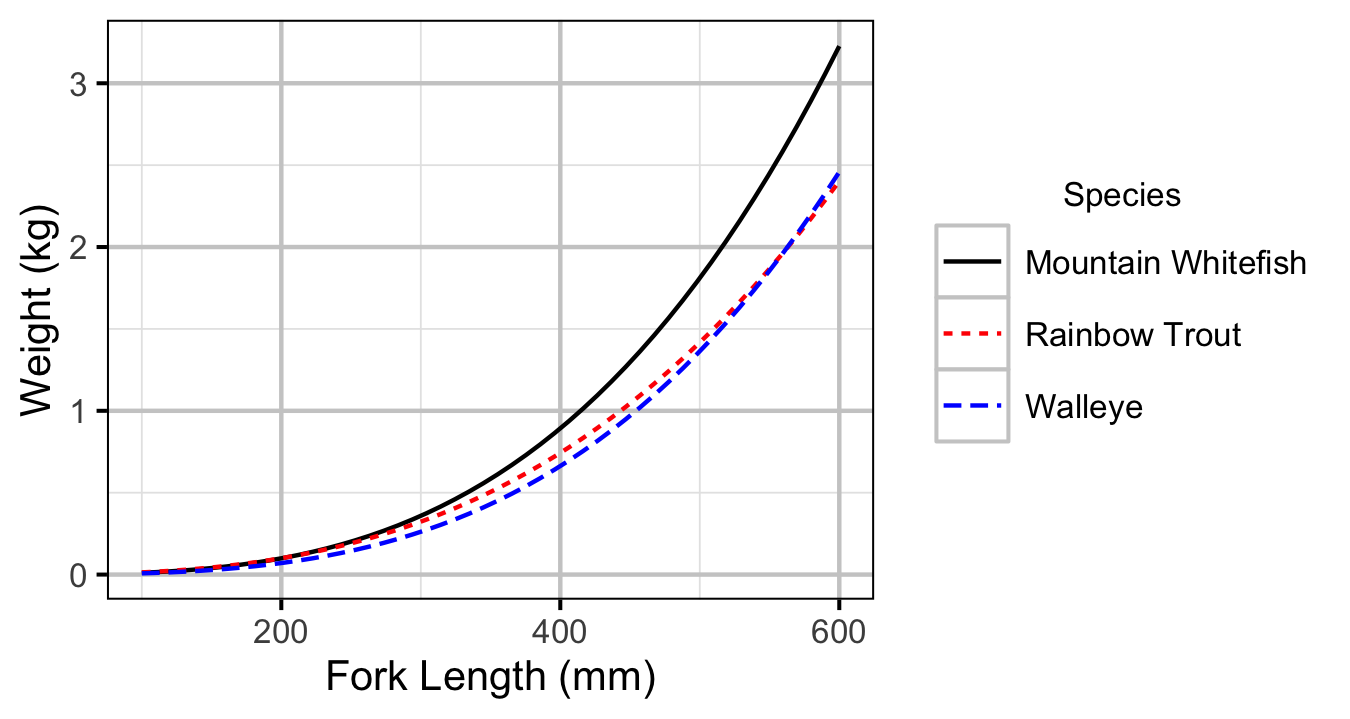
Figure 1. Predicted length-mass relationship by species.
Subadult
Mountain Whitefish
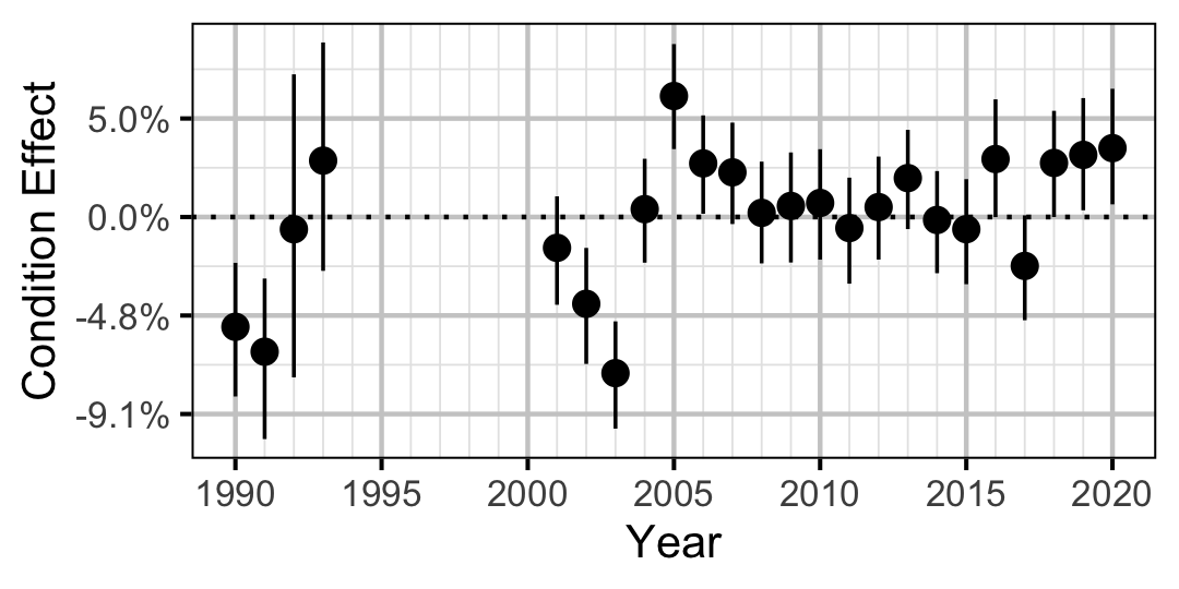
Figure 2. Estimated change in condition relative to a typical year for a 200 mm Mountain Whitefish by year (with 95% CRIs).
Rainbow Trout
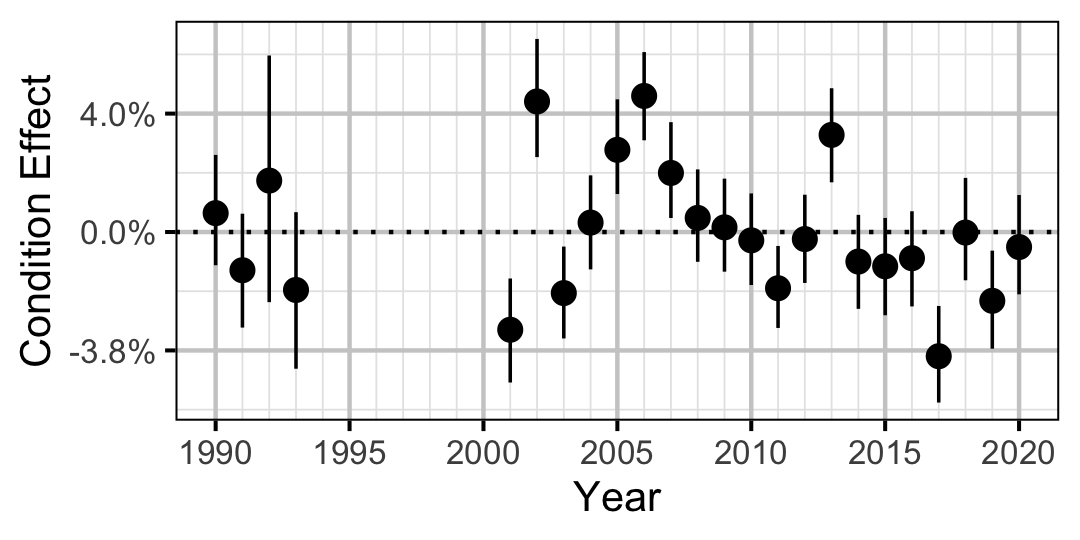
Figure 3. Estimated change in condition relative to a typical year for a 250 mm Rainbow Trout by year (with 95% CRIs).
Adult
Mountain Whitefish
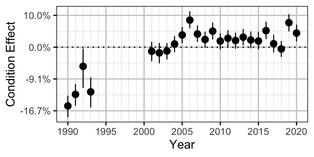
Figure 4. Estimated change in condition relative to a typical year for a 350 mm Mountain Whitefish by year (with 95% CRIs).
Rainbow Trout
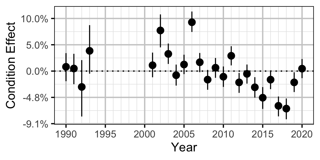
Figure 5. Estimated change in condition relative to a typical year for a 500 mm Rainbow Trout by year (with 95% CRIs).
Walleye
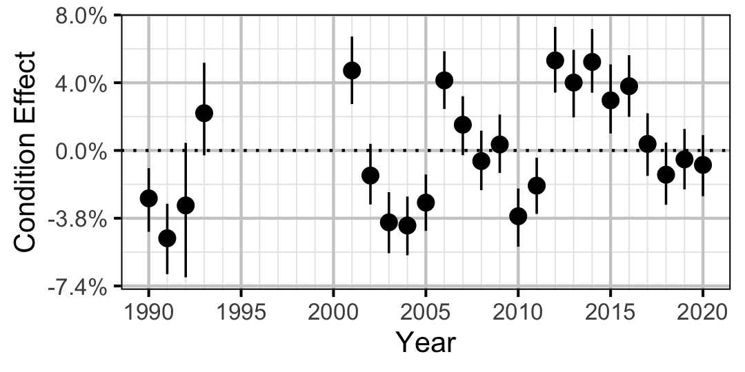
Figure 6. Estimated change in condition relative to a typical year for a 400 mm Walleye by year (with 95% CRIs).
Growth
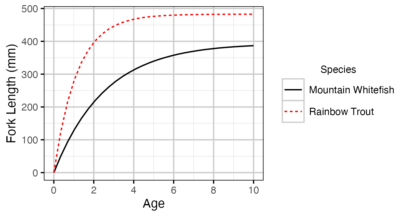
Figure 7. Estimated von Bertalanffy growth curve by species. The growth curve for Walleye is not shown because the growth parameters were not representative for the younger age-classes.
Mountain Whitefish
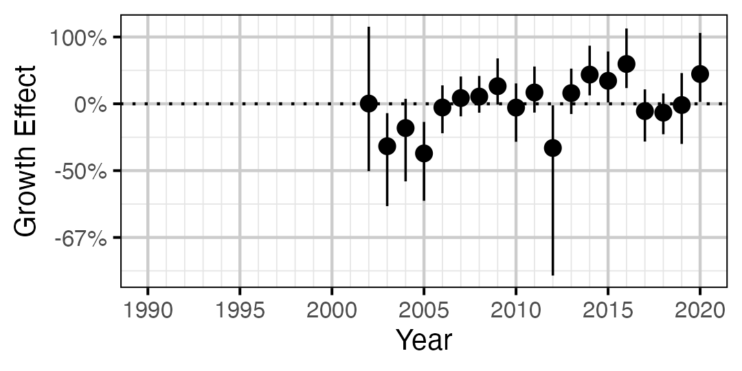
Figure 8. Estimated change in von Bertalanffy growth coefficient (k) relative to a typical year by year (with 95% CIs).
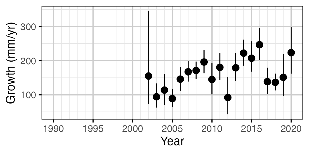
Figure 9. Predicted maximum growth by year (with 95% CIs).
Rainbow Trout
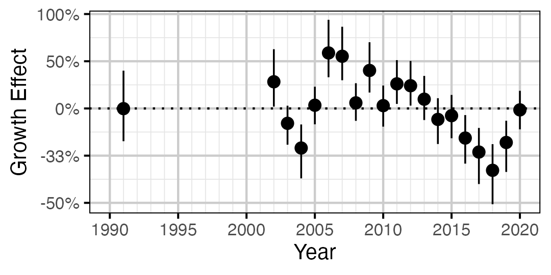
Figure 10. Estimated change in von Bertalanffy growth coefficient (k) relative to a typical year by year (with 95% CIs).
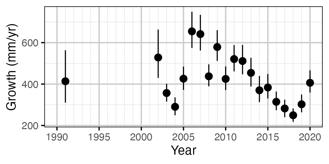
Figure 11. Predicted maximum growth by year (with 95% CIs).
Walleye
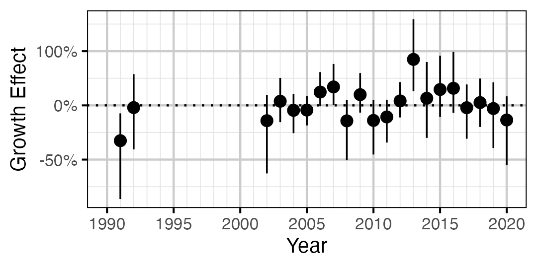
Figure 12. Estimated change in von Bertalanffy growth coefficient (k) relative to a typical year by year (with 95% CIs).
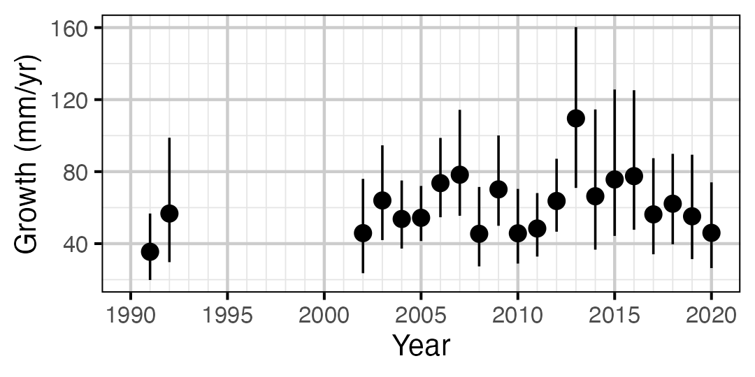
Figure 13. Predicted maximum growth by year (with 95% CIs).
Movement
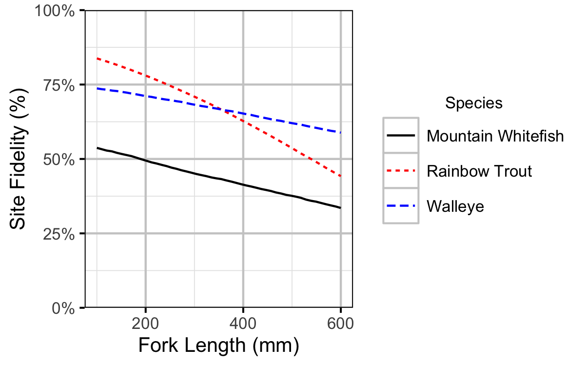
Figure 14. Probability of recapture at the same site versus a different site by fish length (with 95% CRIs).
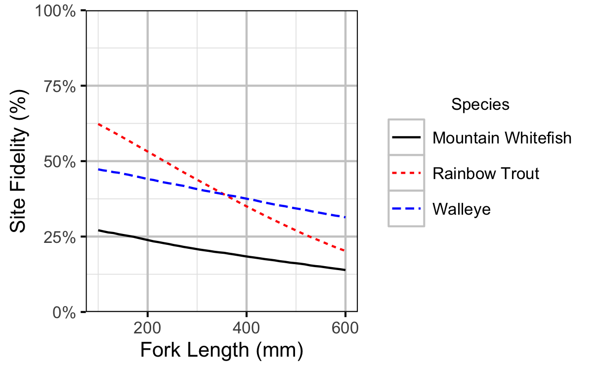
Figure 15. Site fidelity by fish length (with 95% CRIs).
Length-At-Age
Mountain Whitefish
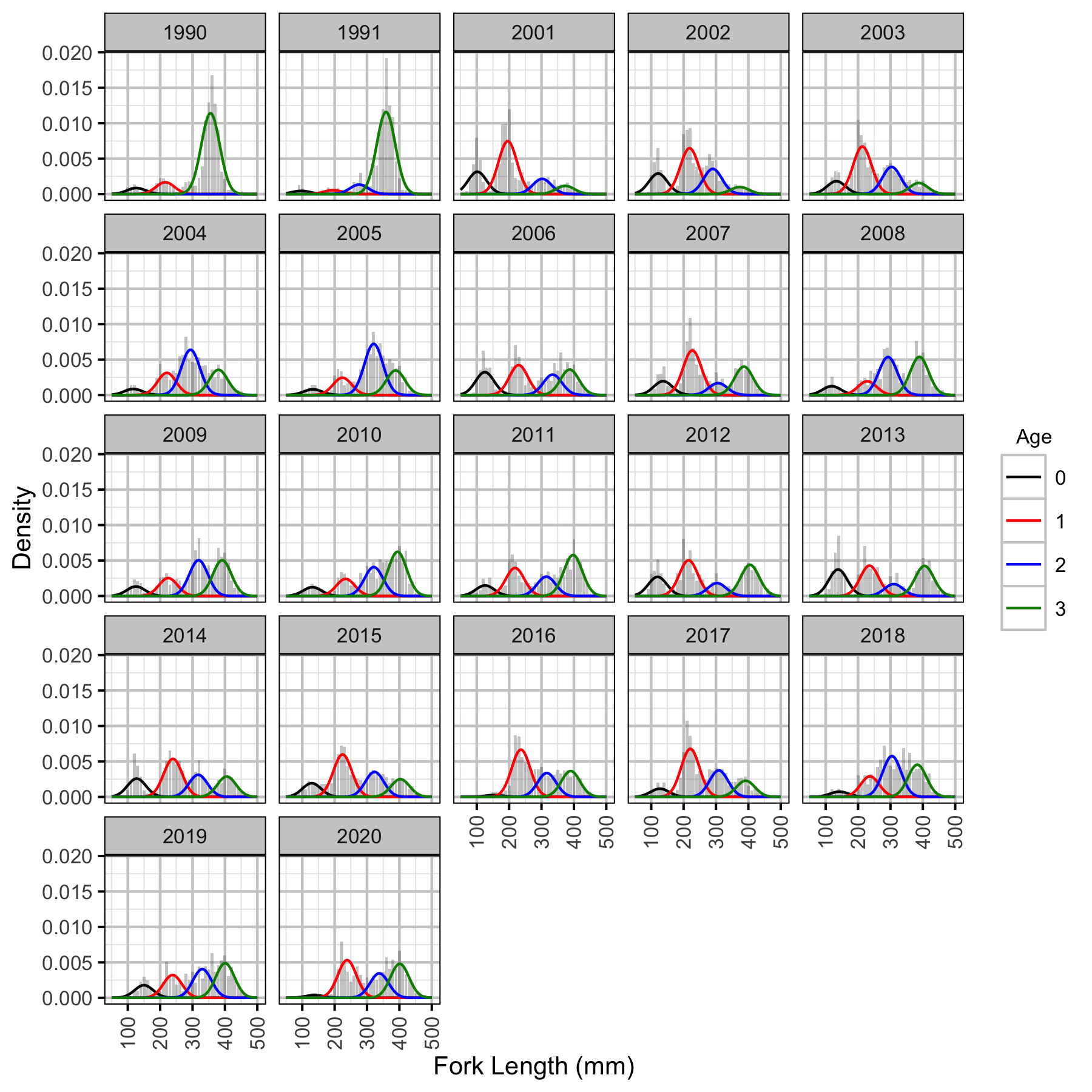
Figure 16. Length-frequency histogram with length-at-age predictions.
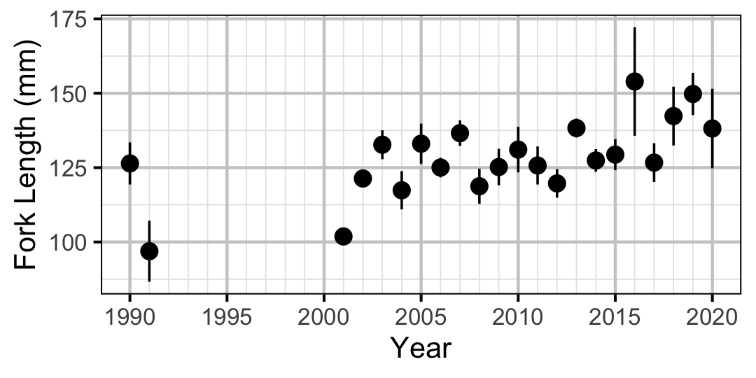
Figure 17. Average length of an age-0 individual by year.
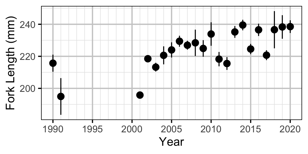
Figure 18. Average length of an age-1 individual by year.
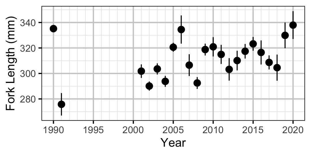
Figure 19. Average length of an age-2 individual by year.
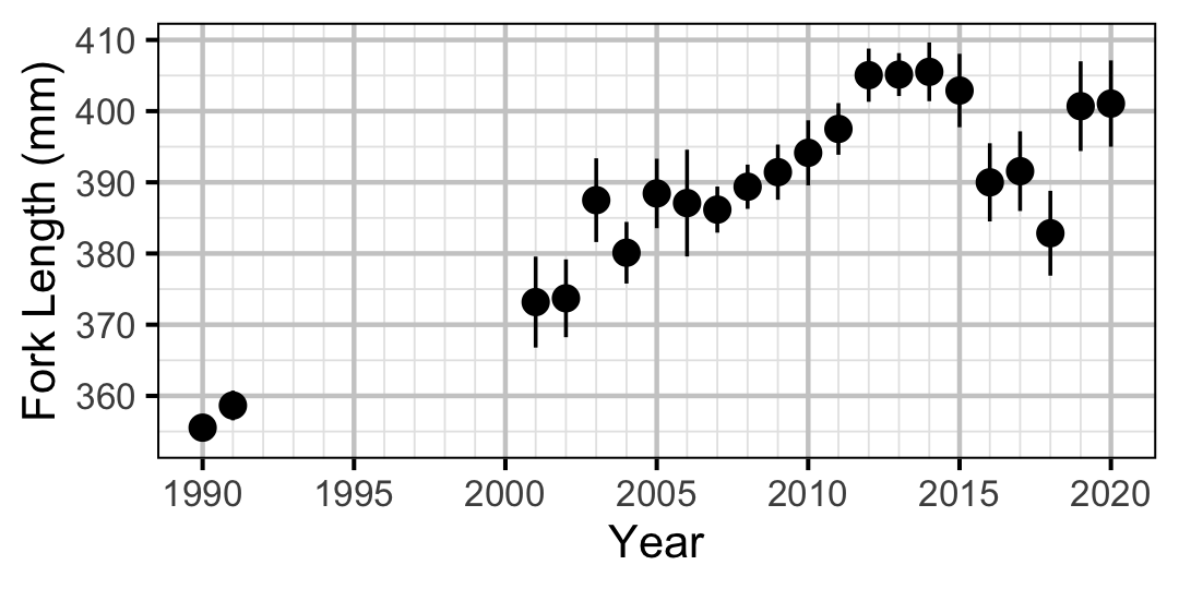
Figure 20. Average length of an age-3+ individual by year.
Rainbow Trout
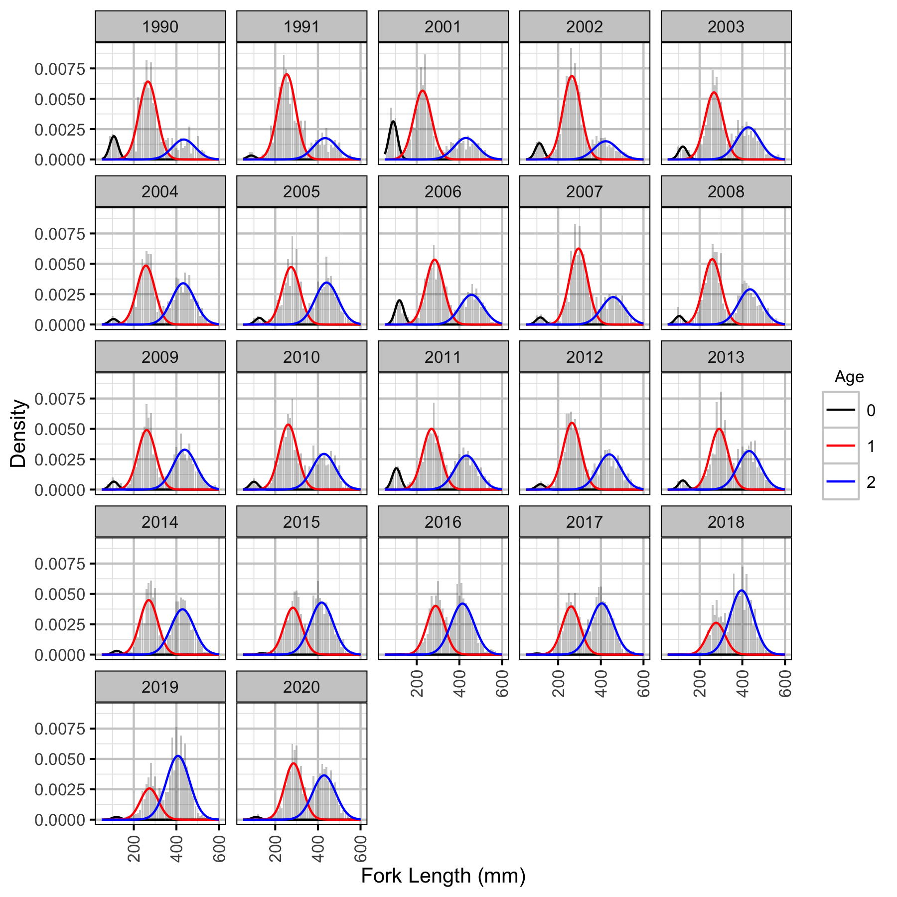
Figure 21. Length-frequency histogram with length-at-age predictions.
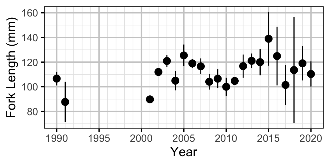
Figure 22. Average length of an age-0 individual by year.
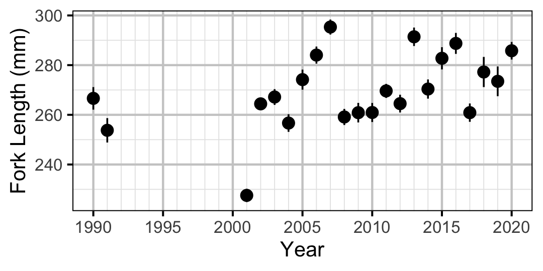
Figure 23. Average length of an age-1 individual by year.
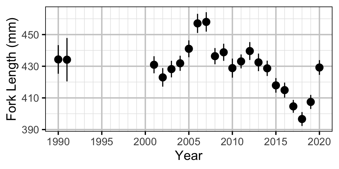
Figure 24. Average length of an age-2+ individual by year.
Survival
Adult
Mountain Whitefish
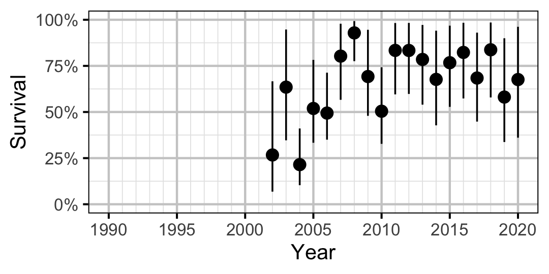
Figure 25. Predicted annual survival for an adult Mountain Whitefish.
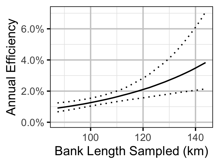
Figure 26. Predicted annual efficiency for an adult Mountain Whitefish.
Rainbow Trout
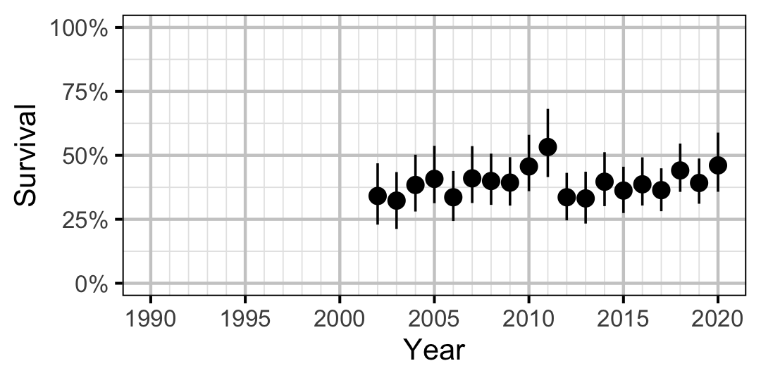
Figure 27. Predicted annual survival for an adult Rainbow Trout.
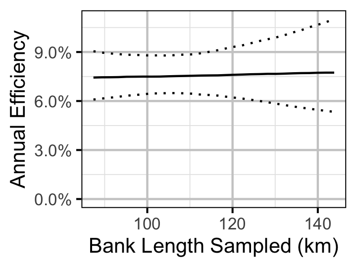
Figure 28. Predicted annual efficiency for an adult Rainbow Trout.
Walleye
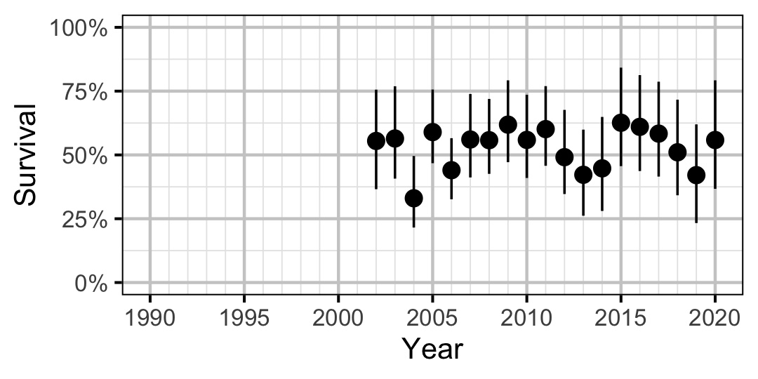
Figure 29. Predicted annual survival for an adult Walleye.
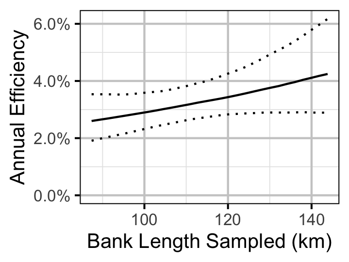
Figure 30. Predicted annual efficiency for an adult Walleye.
Observer Length Correction
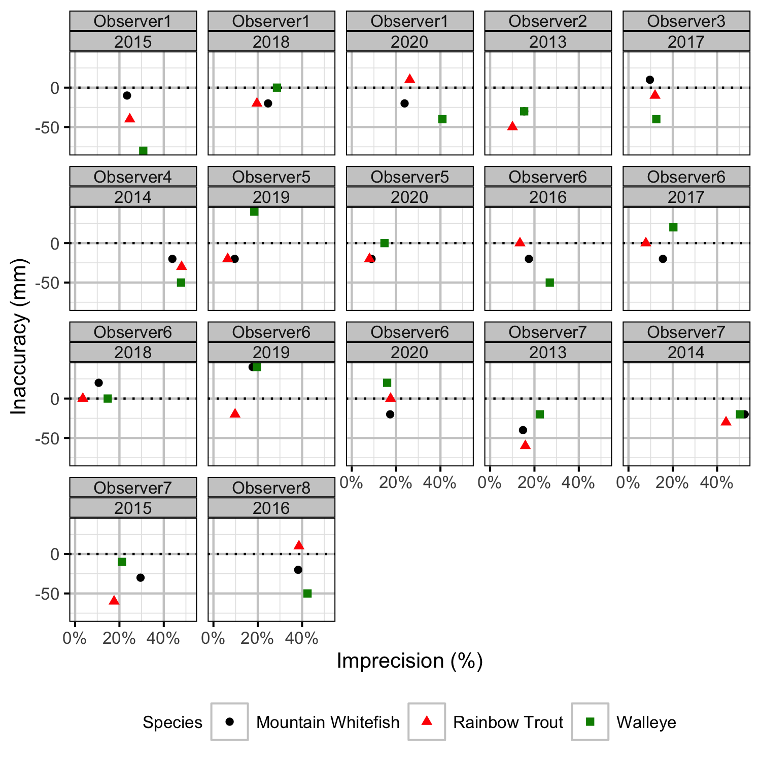
Figure 31. Length inaccuracy and imprecision by observer, year and species.
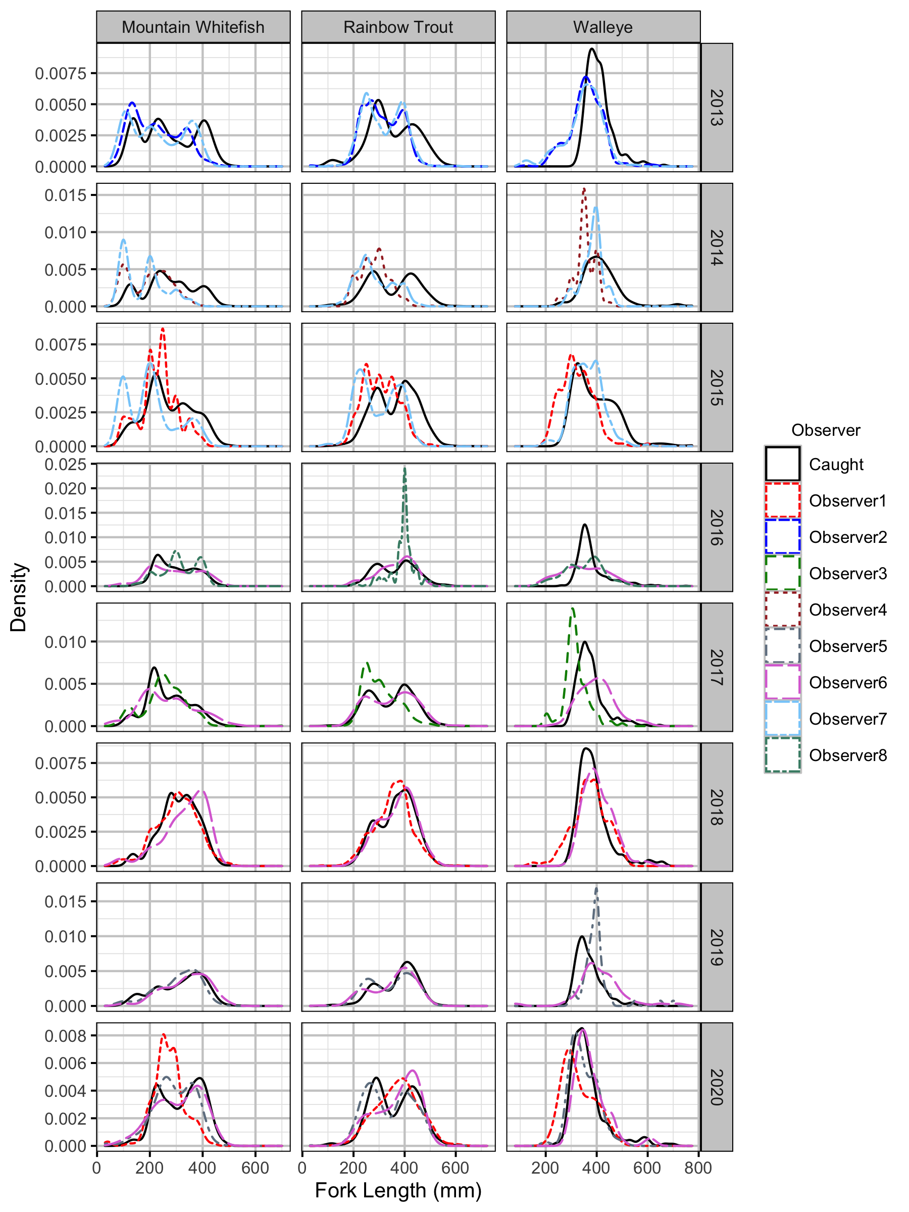
Figure 32. Uncorrected length density plots by species, year and observer.
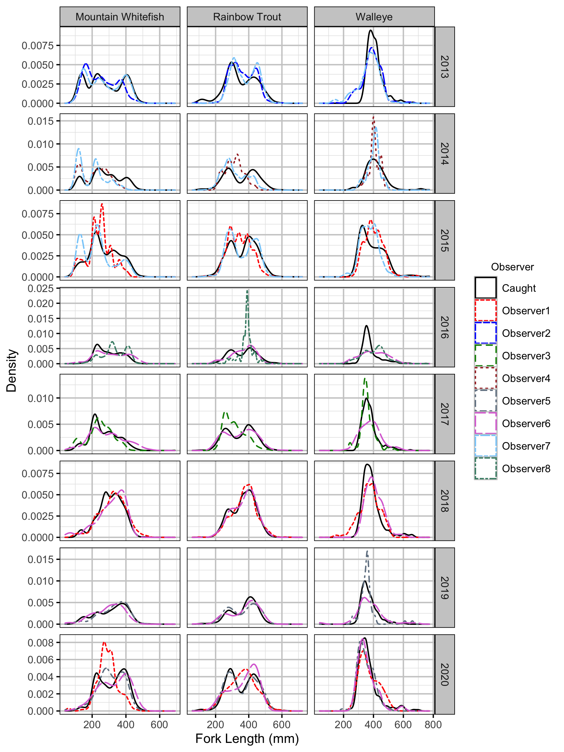
Figure 33. Corrected length density plots by species, year and observer.
Capture Efficiency
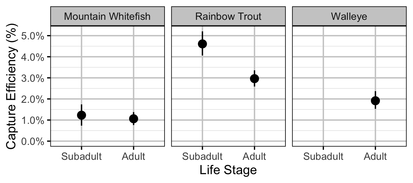
Figure 34. Predicted capture efficiency by species and life stage (with 95% CRIs).
Mountain Whitefish
Subadult
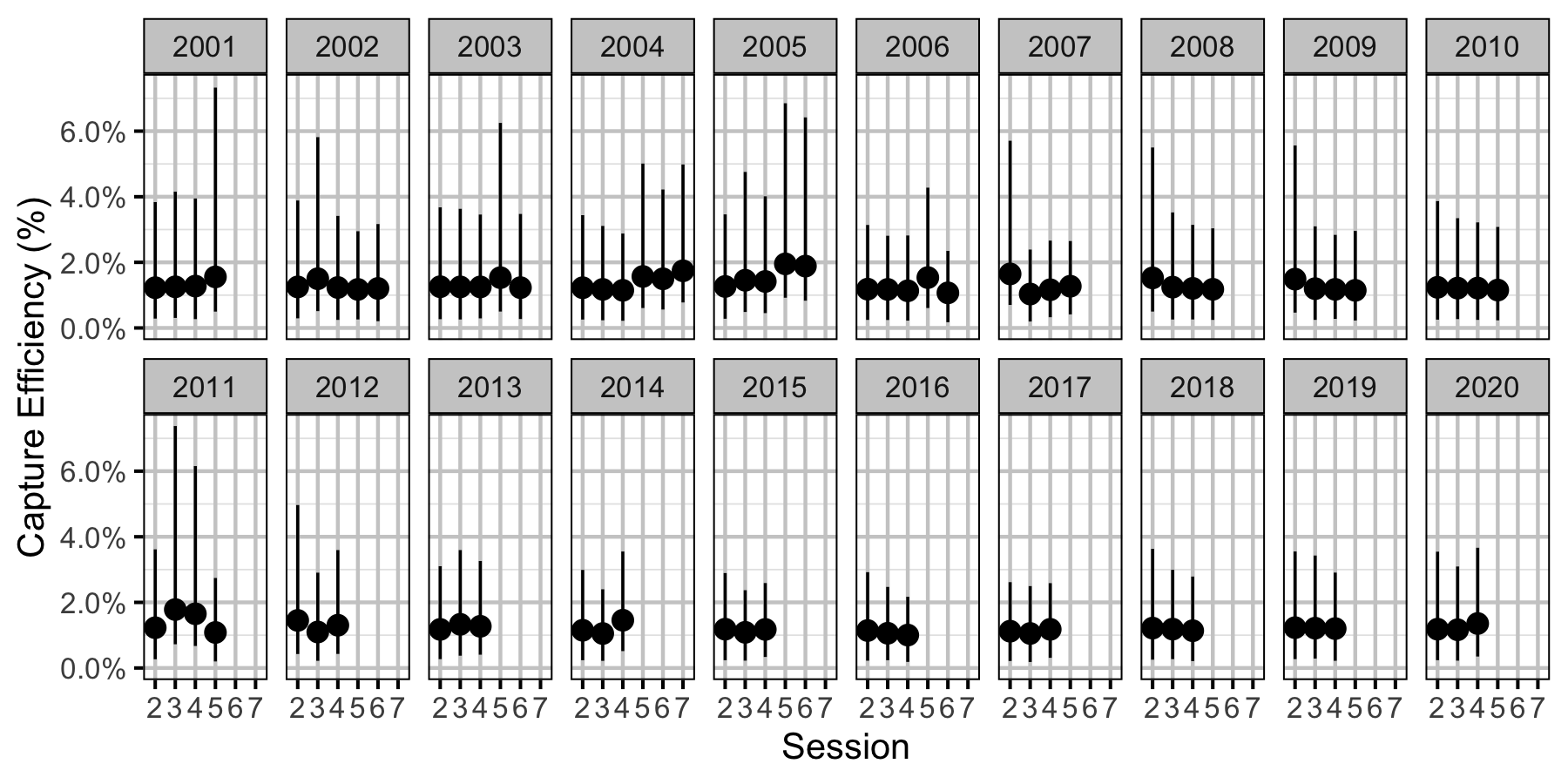
Figure 35. Predicted capture efficiency for a subadult Mountain Whitefish by session and year (with 95% CRIs).
Adult
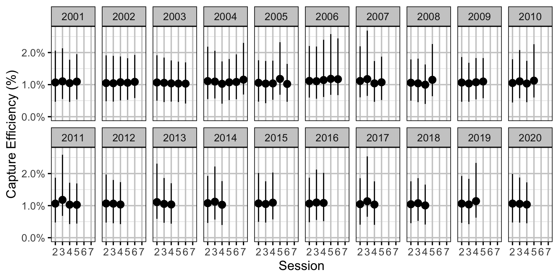
Figure 36. Predicted capture efficiency for an adult Mountain Whitefish by session and year (with 95% CRIs).
Rainbow Trout
Subadult
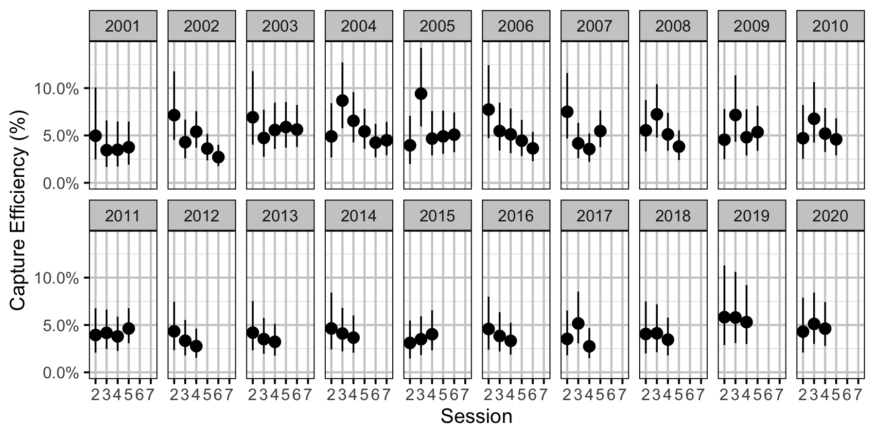
Figure 37. Predicted capture efficiency for a subadult Rainbow Trout by session and year (with 95% CRIs).
Adult
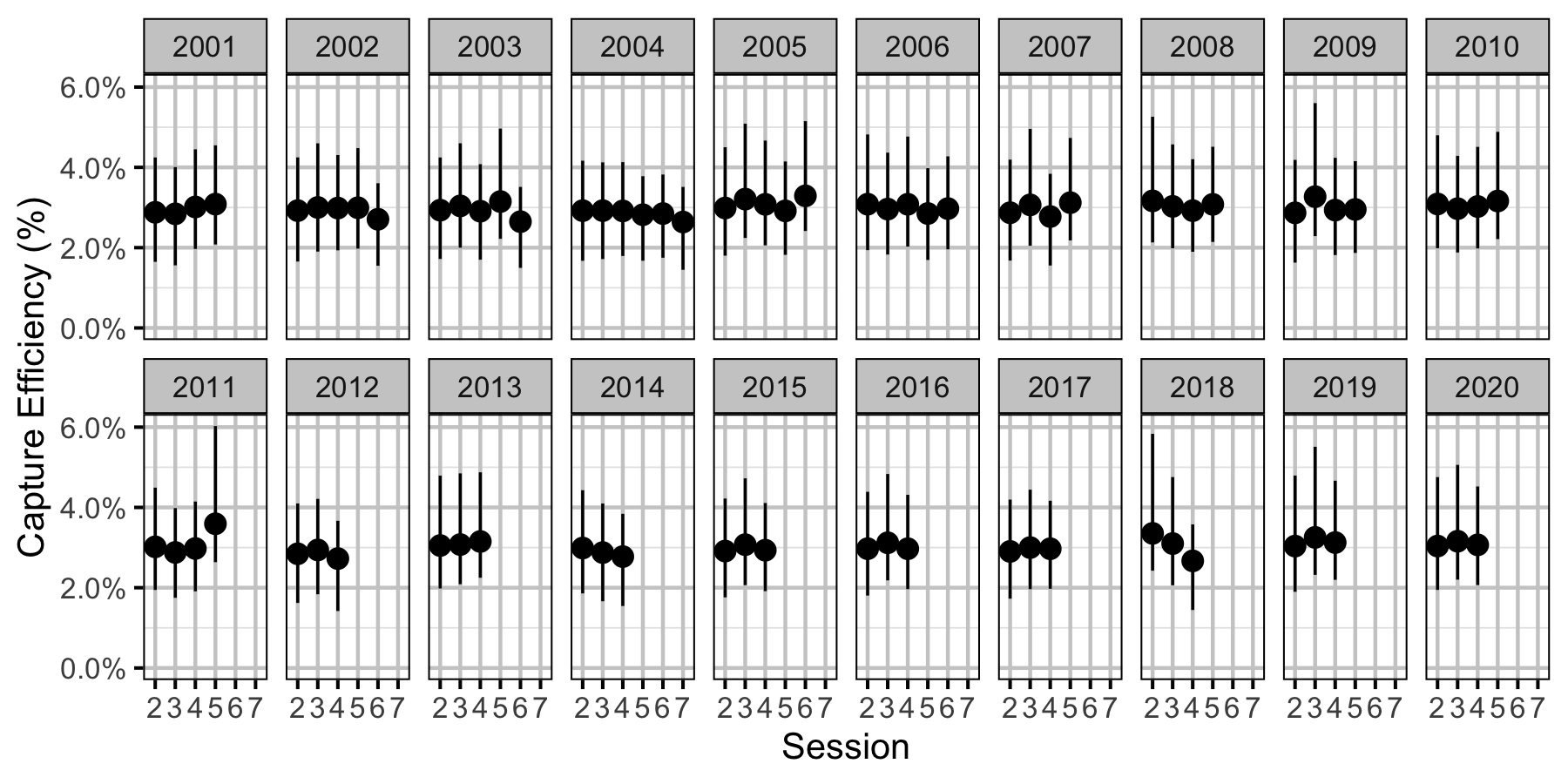
Figure 38. Predicted capture efficiency for an adult Rainbow Trout by session and year (with 95% CRIs).
Walleye
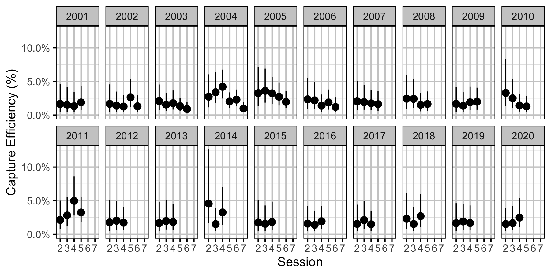
Figure 39. Predicted capture efficiency for an adult Walleye by session and year (with 95% CRIs).
Abundance
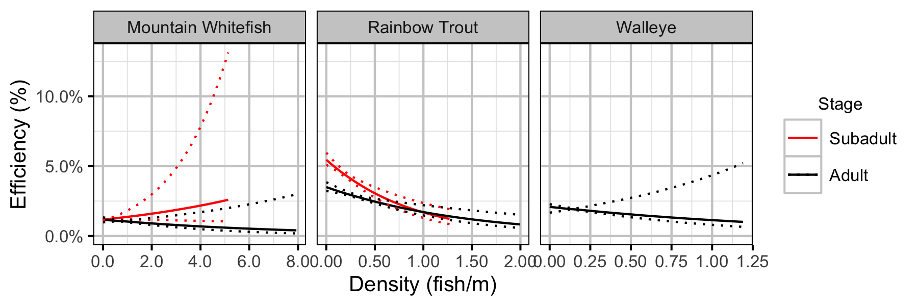
Figure 40. Effect of density on capture efficiency by species and stage (with 95% CIs).
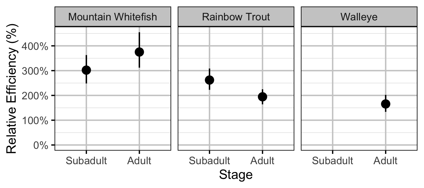
Figure 41. Effect of counting (versus capture) on encounter efficiency at typical density by species and stage (with 95% CIs).
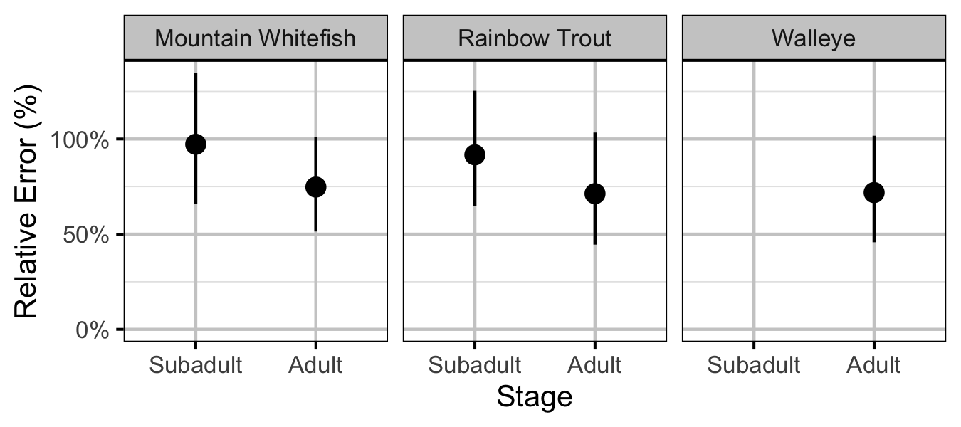
Figure 42. Effect of counting (versus capture) on overdispersion by species and stage (with 95% CIs).
Mountain Whitefish
Subadult
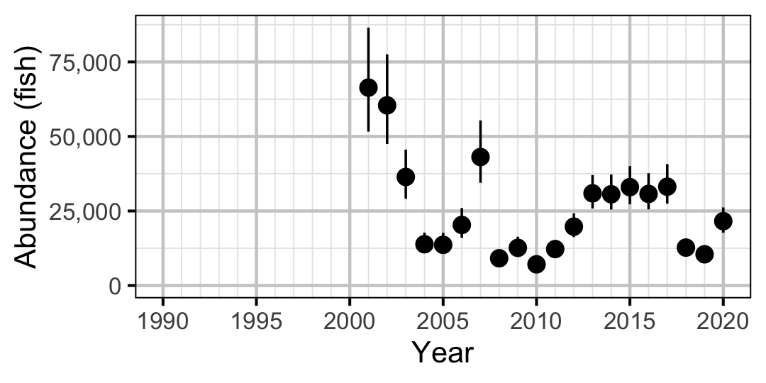
Figure 43. Estimated abundance of subadult Mountain Whitefish by year (with 95% CIs).
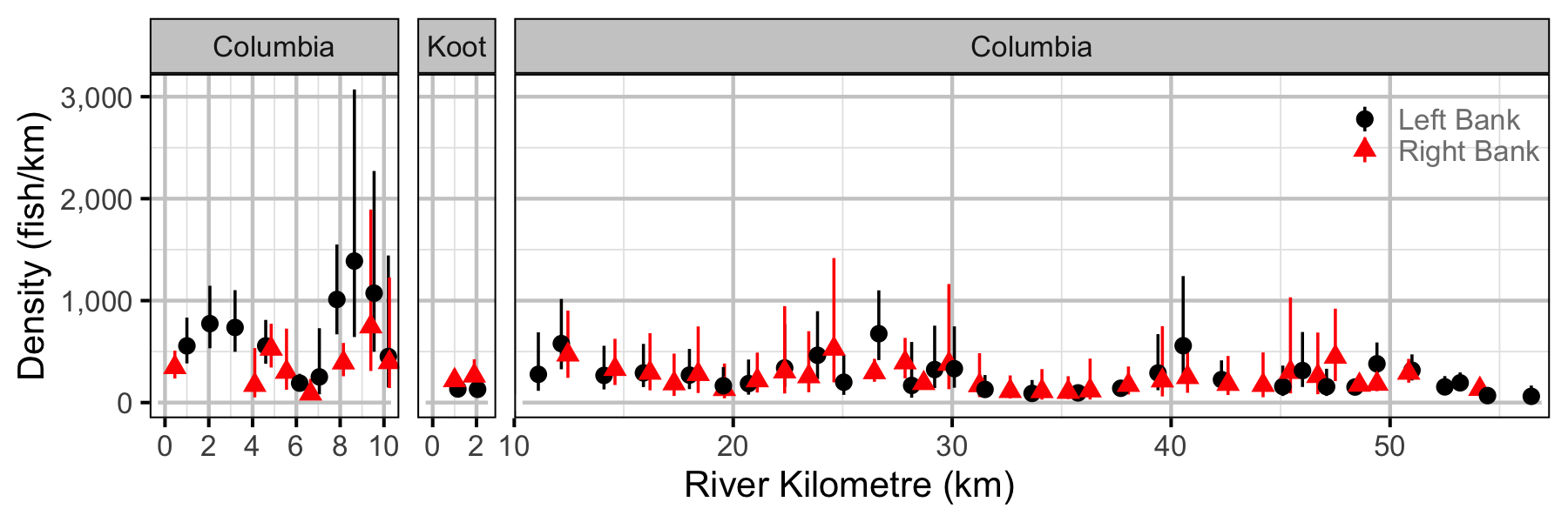
Figure 44. Estimated lineal river count density of subadult Mountain Whitefish by site in (with 95% CIs).
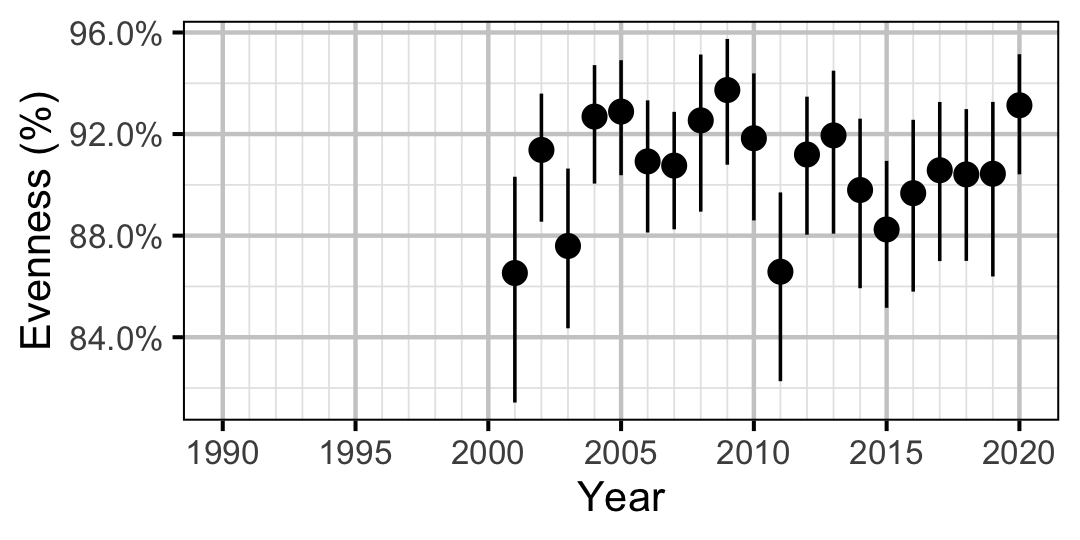
Figure 45. Estimated evenness of subadult Mountain Whitefish at index sites by year (with 95% CIs).
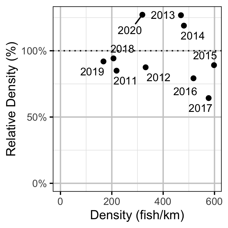
Figure 46. Estimated density of subadult Mountain Whitefish at non-index relative to index sites by year.
Adult
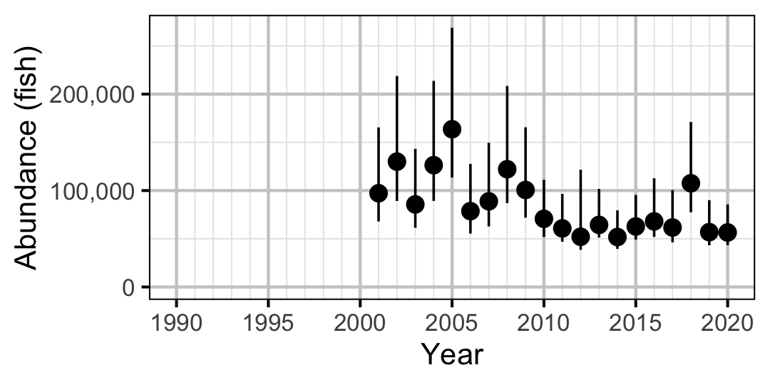
Figure 47. Estimated abundance of adult Mountain Whitefish by year (with 95% CIs).
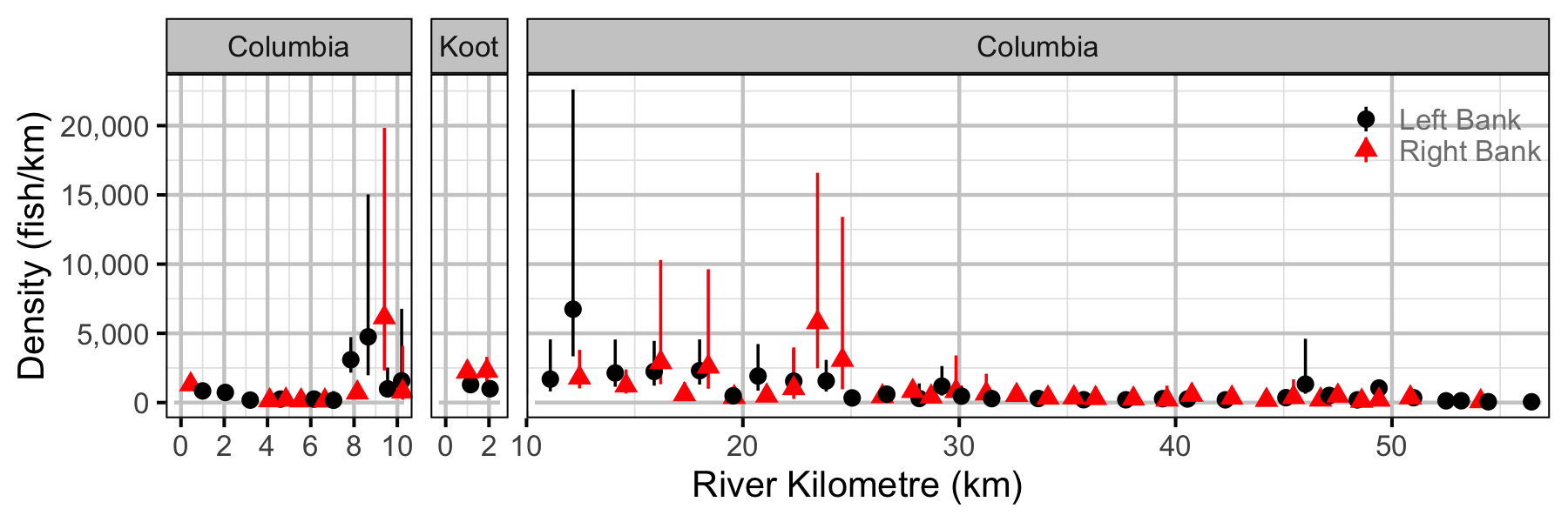
Figure 48. Estimated lineal river count density of adult Mountain Whitefish by site in (with 95% CIs).
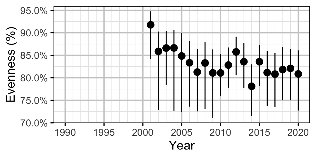
Figure 49. Estimated evenness of adult Mountain Whitefish at index sites by year (with 95% CIs).
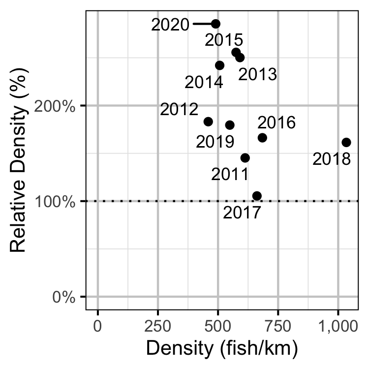
Figure 50. Estimated density of adult Mountain Whitefish at non-index relative to index sites by year.
Rainbow Trout
Subadult
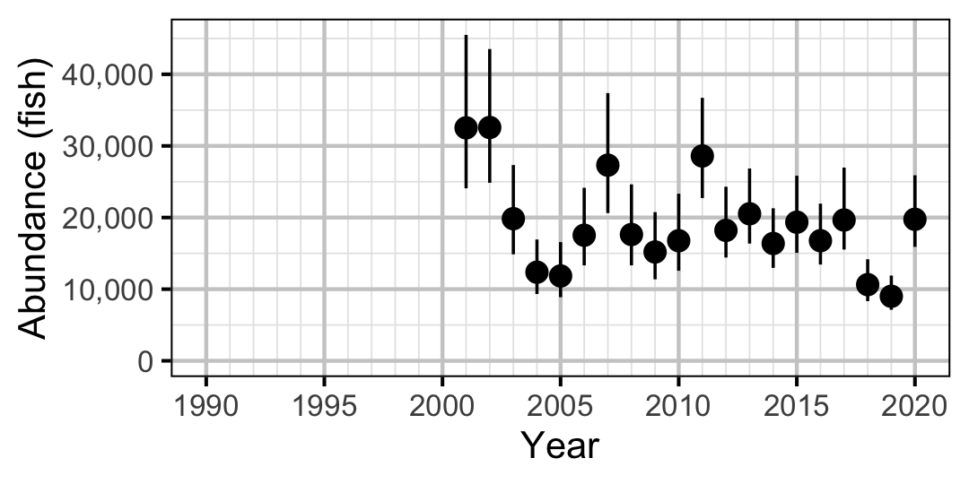
Figure 51. Estimated abundance of subadult Rainbow Trout by year (with 95% CIs).
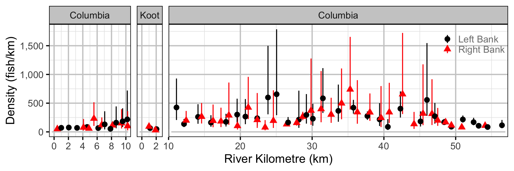
Figure 52. Estimated lineal river count density of subadult Rainbow Trout by site in (with 95% CIs).
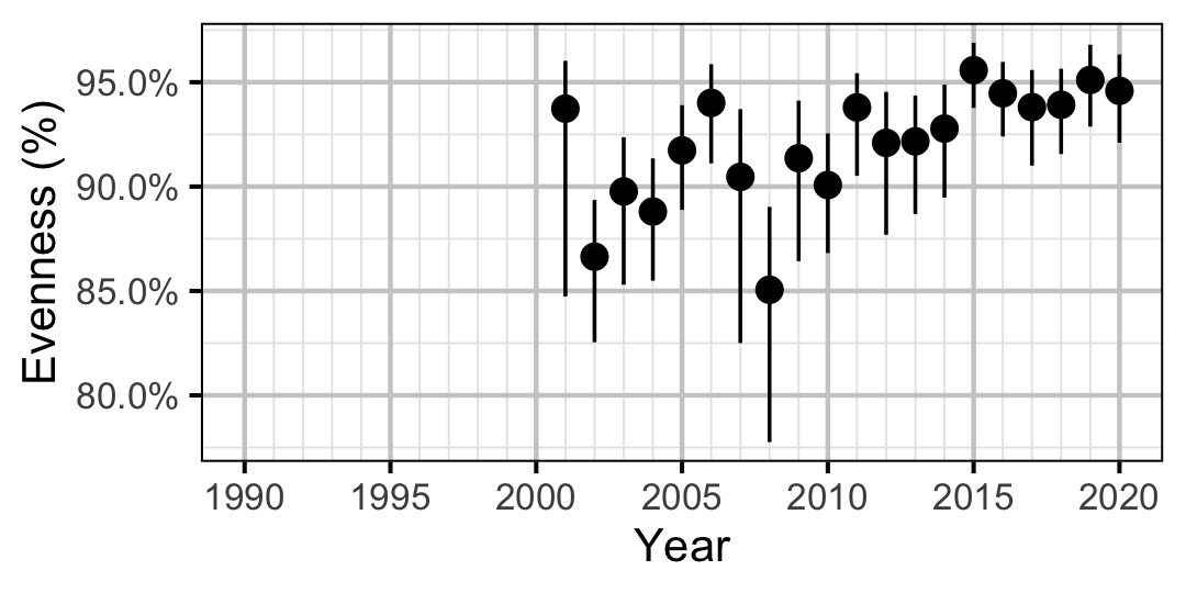
Figure 53. Estimated evenness of subadult Rainbow Trout at index sites by year (with 95% CIs).
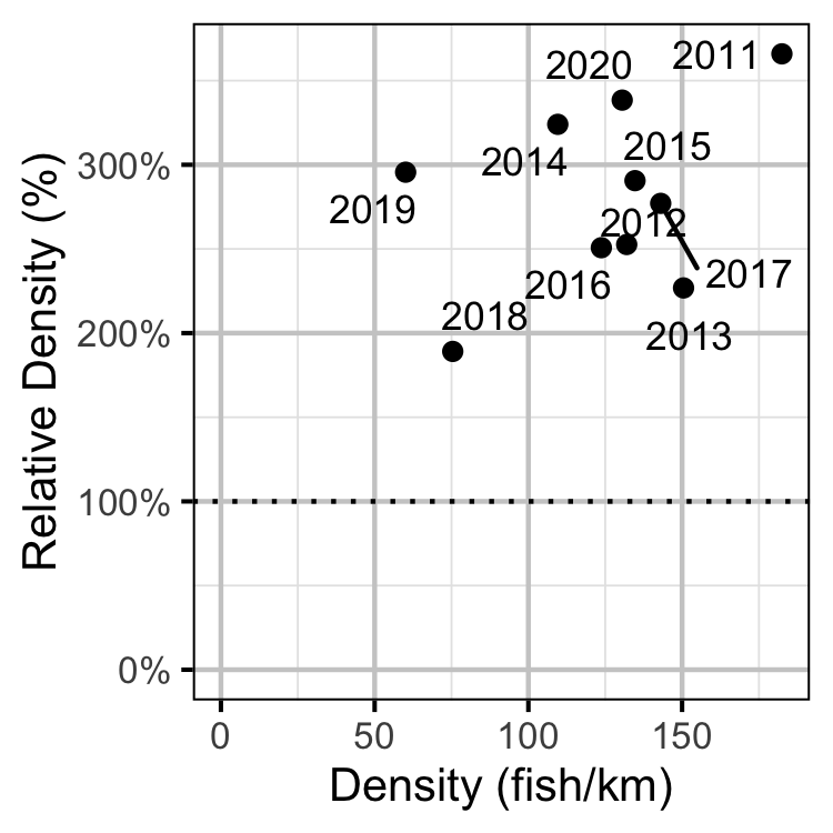
Figure 54. Estimated density of subadult Rainbow Trout at non-index relative to index sites by year.
Adult
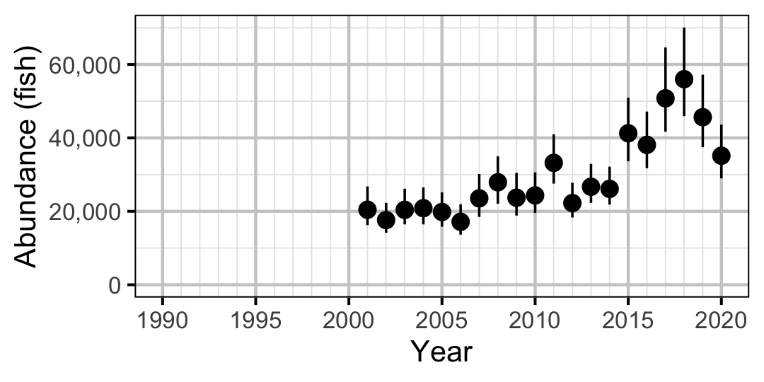
Figure 55. Estimated abundance of adult Rainbow Trout by year (with 95% CIs).
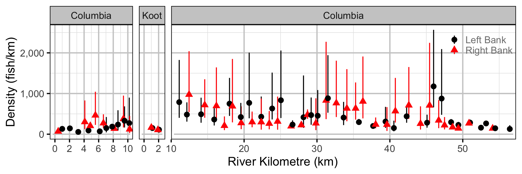
Figure 56. Estimated lineal river count density of adult Rainbow Trout by site in (with 95% CIs).
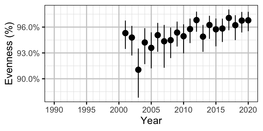
Figure 57. Estimated evenness of adult Rainbow Trout at index sites by year (with 95% CIs).
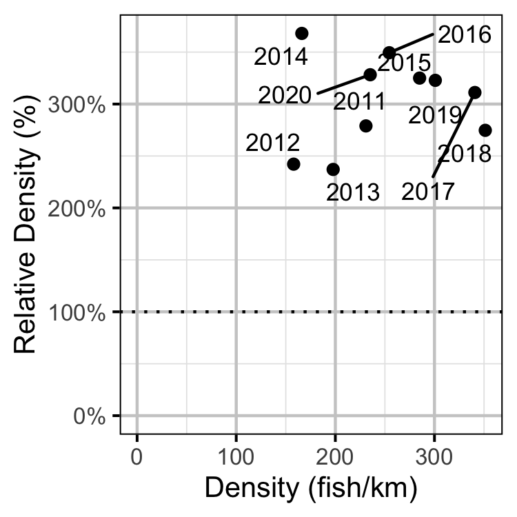
Figure 58. Estimated density of adult Rainbow Trout at non-index relative to index sites by year.
Walleye
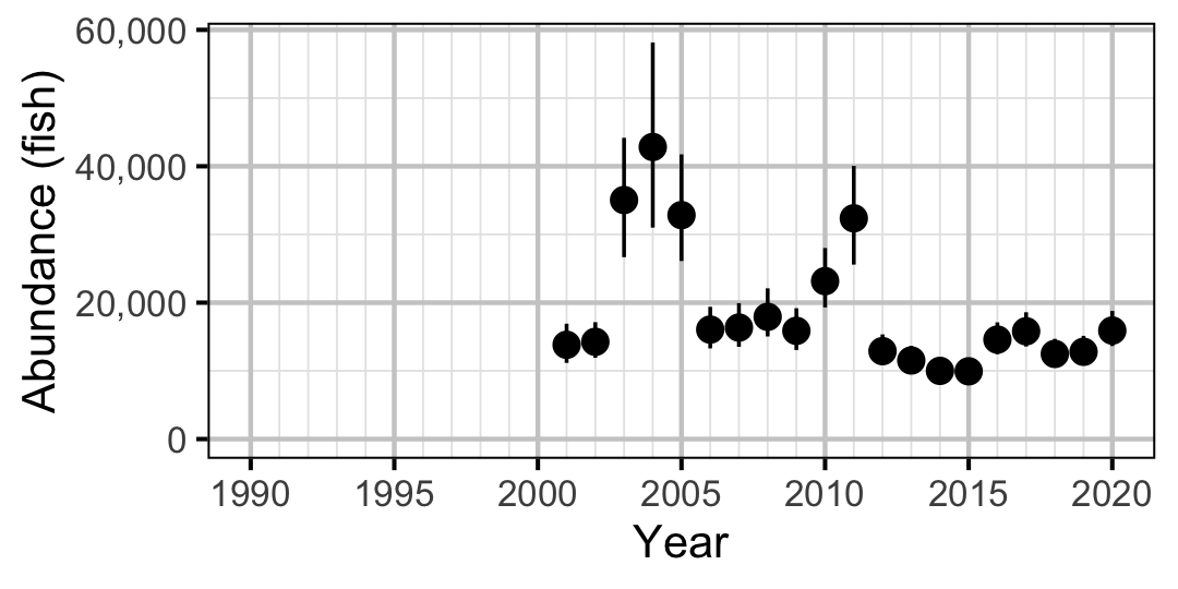
Figure 59. Estimated abundance of adult Walleye by year (with 95% CIs).
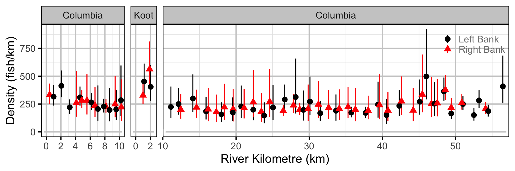
Figure 60. Estimated lineal river count density of adult Walleye by site in (with 95% CIs).
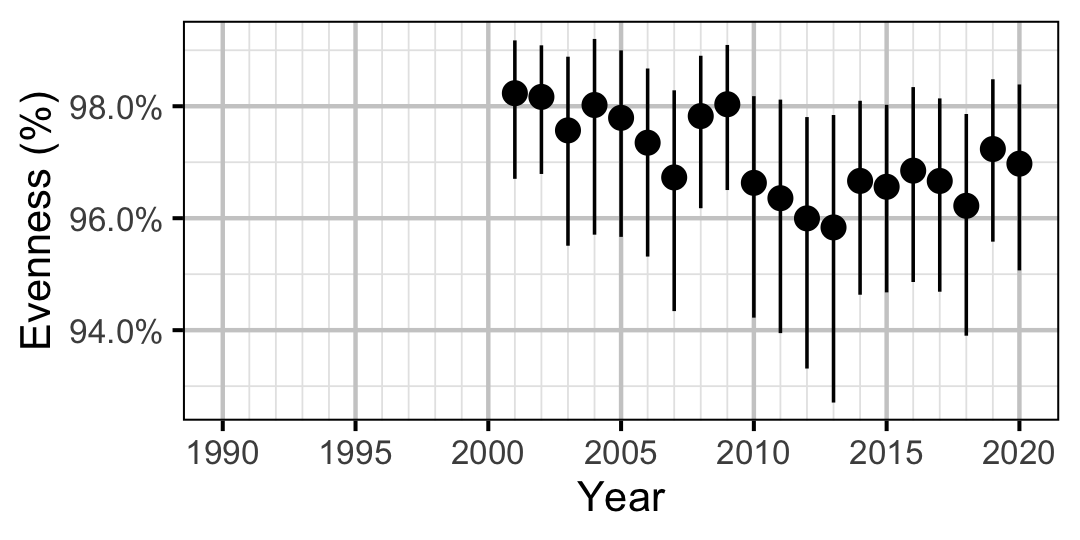
Figure 61. Estimated evenness of adult Walleye at index sites by year (with 95% CIs).
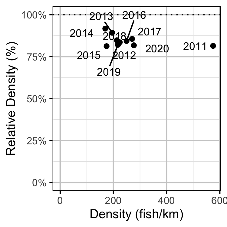
Figure 62. Estimated density of adult Walleye at non-index relative to index sites by year.
Survival (Abundance-based)
Mountain Whitefish
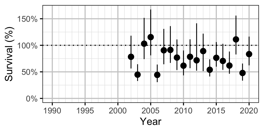
Figure 63. Predicted annual survival for adult and subadult Mountain Whitefish.
Rainbow Trout
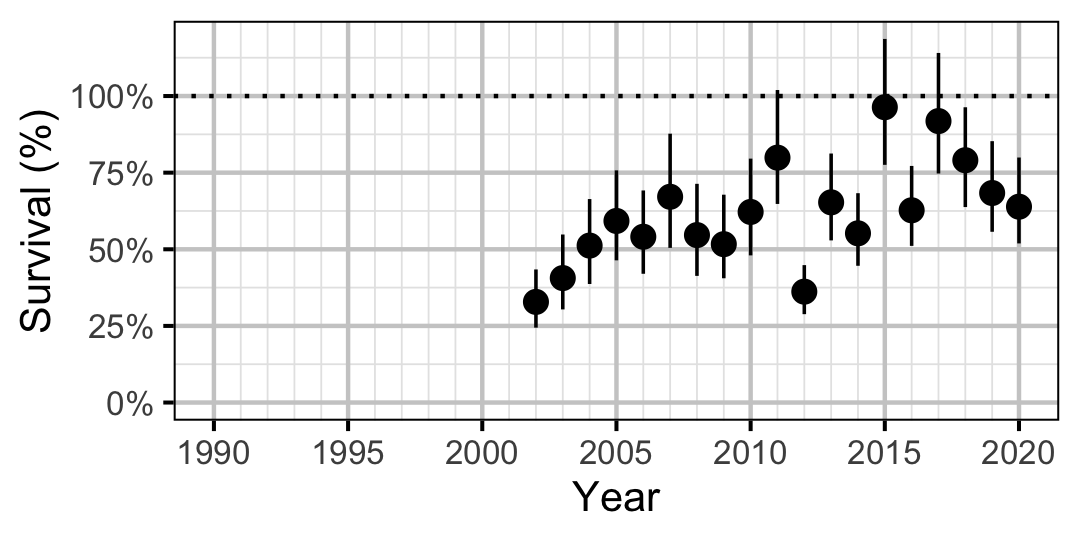
Figure 64. Predicted annual survival for adult and subadult Rainbow Trout.
Weight
Mountain Whitefish
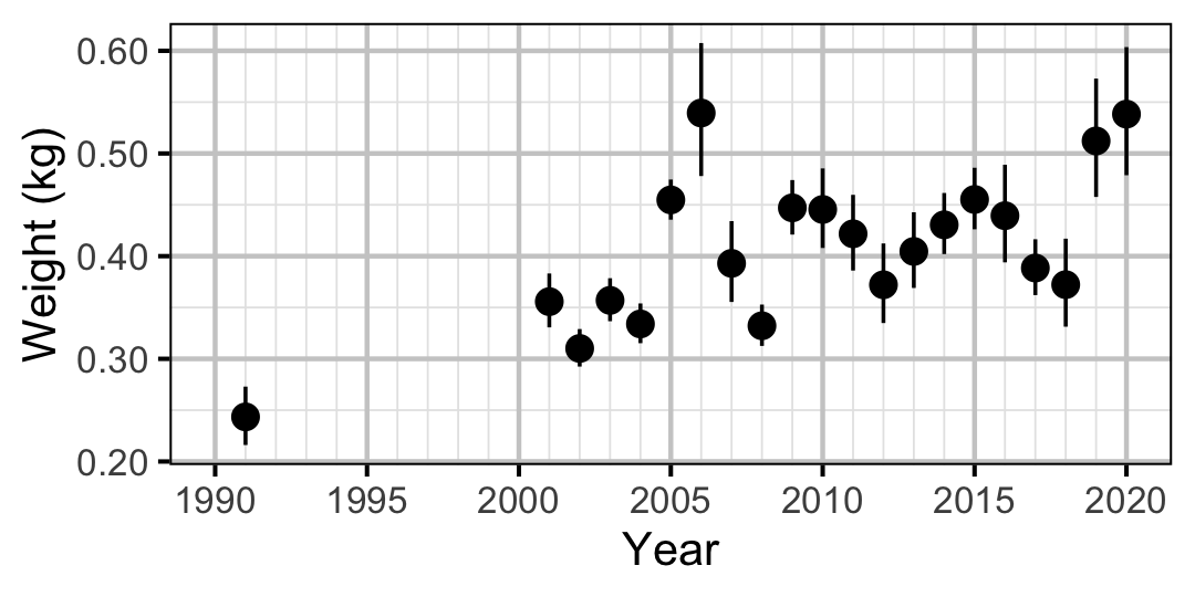
Figure 65. Predicted weight of an adult Mountain Whitefish by year (with 95% CIs).
Rainbow Trout
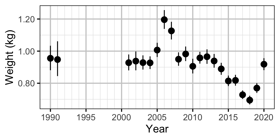
Figure 66. Predicted weight of an adult Rainbow Trout by year (with 95% CIs).
Fecundity
Mountain Whitefish
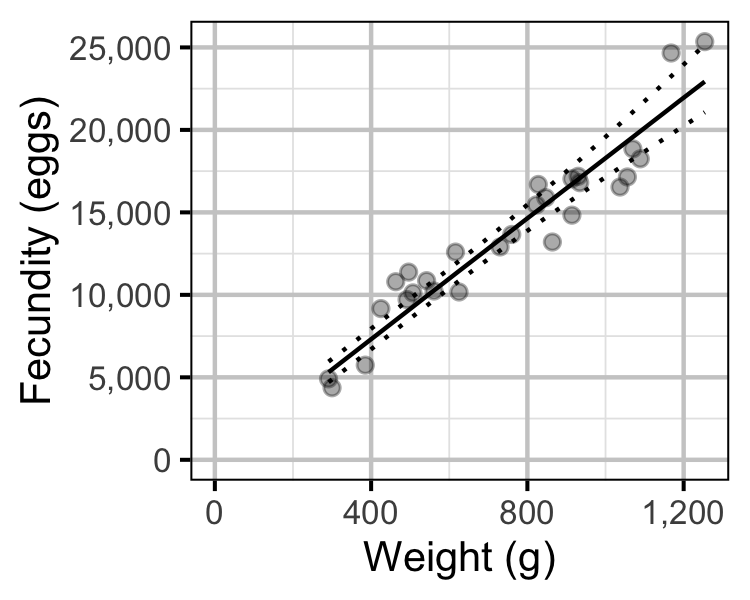
Figure 67. The fecundity-weight relationship for Mountain Whitefish (with 95% CRIs). The data are from Boyer et al (2017).
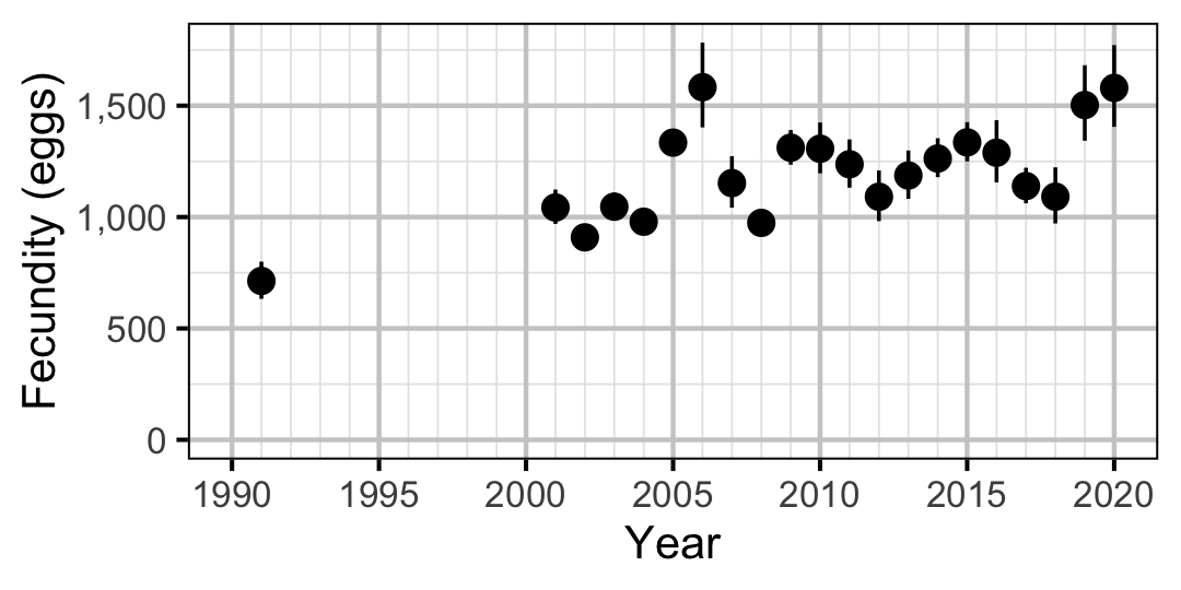
Figure 68. Predicted fecundity of an adult female Mountain Whitefish by year (with 95% CIs).
Rainbow Trout
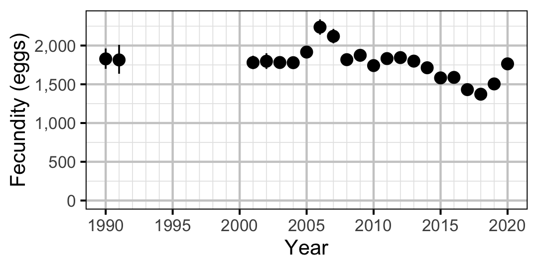
Figure 69. Predicted fecundity of an adult female Rainbow Trout by year (with 95% CIs).
Egg Deposition
Mountain Whitefish
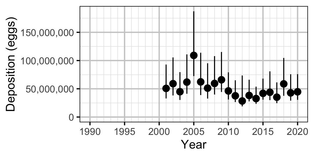
Figure 70. Predicted total egg deposition by Mountain Whitefish by year (with 95% CIs).
Rainbow Trout
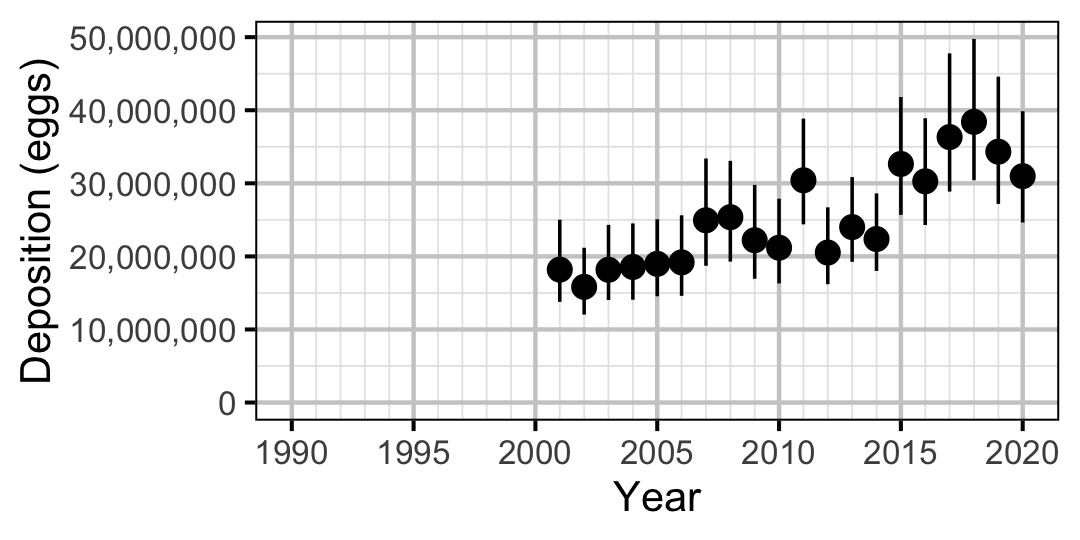
Figure 71. Predicted total egg deposition by Rainbow Trout by year (with 95% CIs).
Stock-Recruitment
Mountain Whitefish
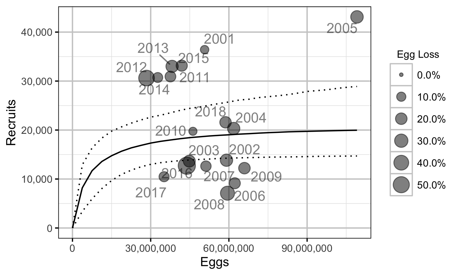
Figure 72. Predicted stock-recruitment relationship by spawn year (with 95% CRIs).
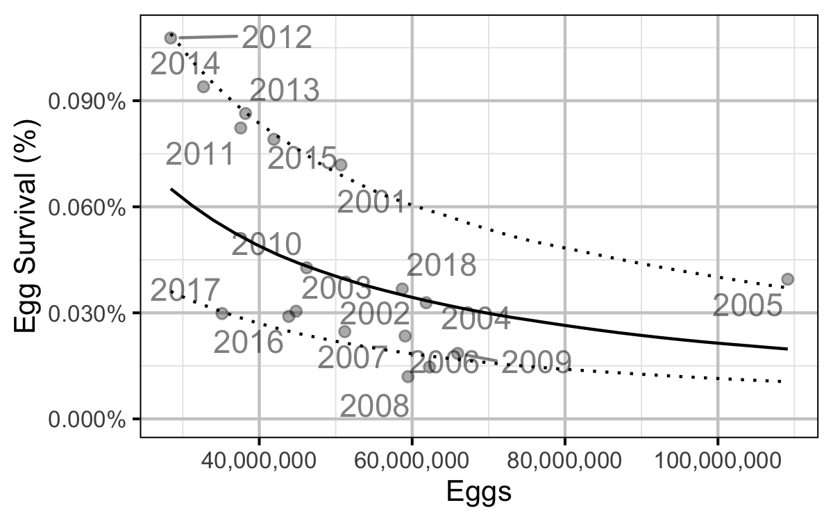
Figure 73. Predicted egg to age-1 survival by total egg deposition (with 95% CRIs).
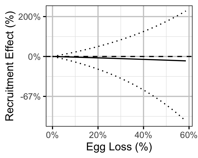
Figure 74. Predicted effect of egg loss on the number of age-1 recruits (with 95% CRIs).
Rainbow Trout
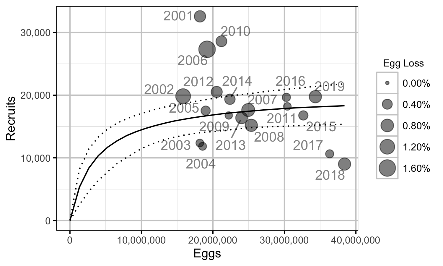
Figure 75. Predicted stock-recruitment relationship by spawn year (with 95% CRIs).
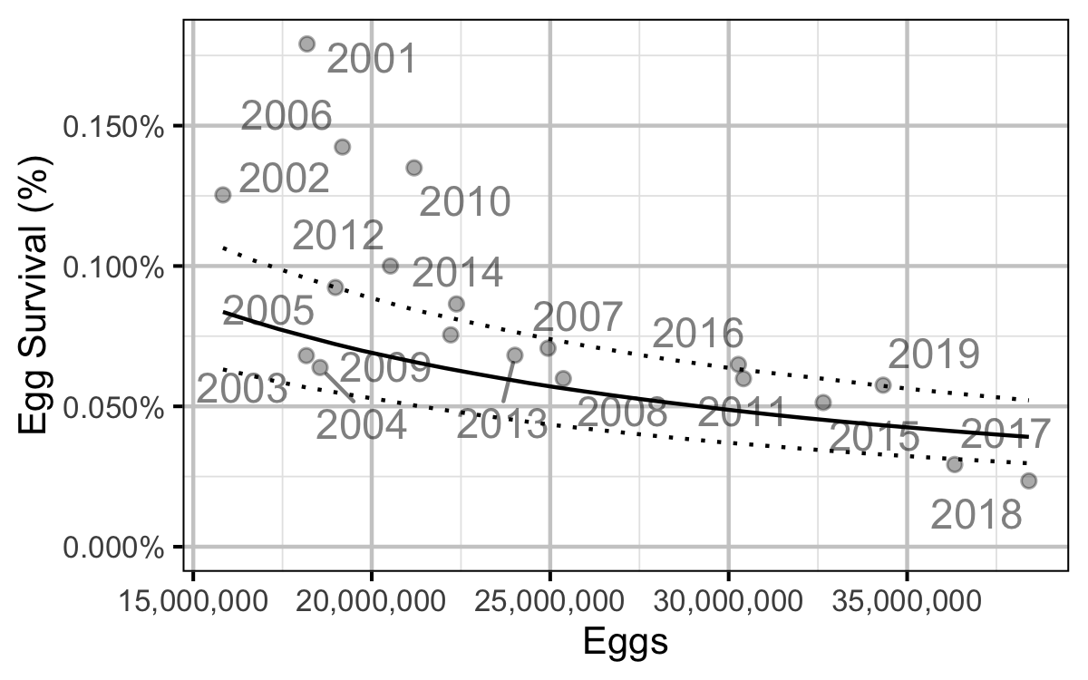
Figure 76. Predicted egg to age-1 survival by total egg deposition (with 95% CRIs).
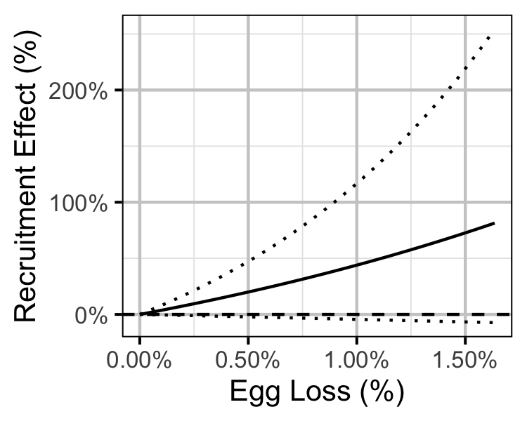
Figure 77. Predicted effect of egg loss on the number of age-1 recruits (with 95% CRIs).
Age-Ratios
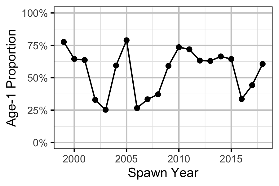
Figure 78. Proportion of Age-1 Mountain Whitefish by spawn year.
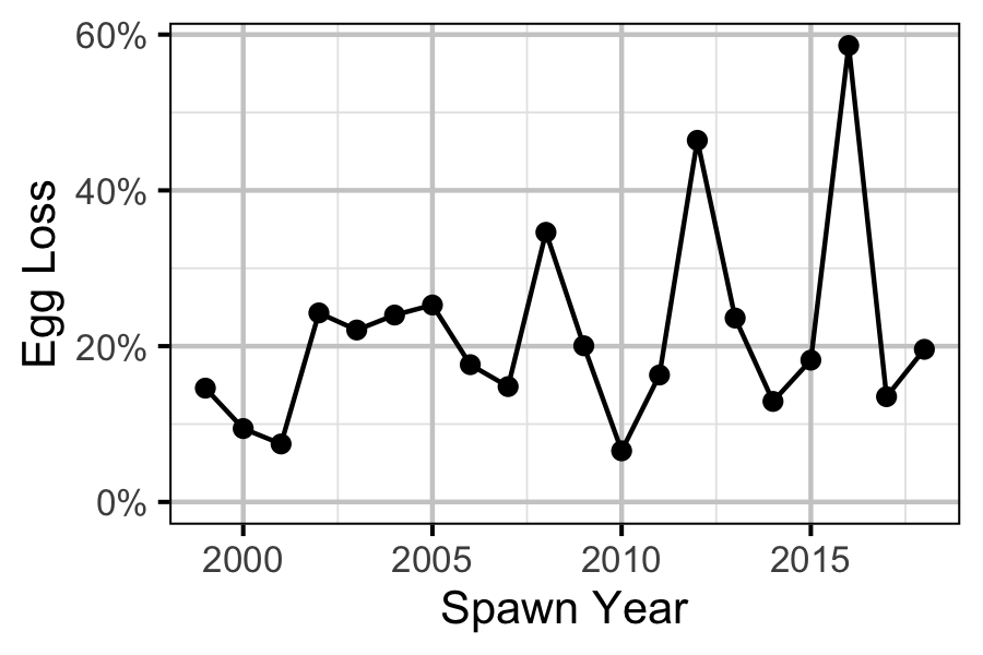
Figure 79. Percentage Mountain Whitefish egg loss by spawn year.
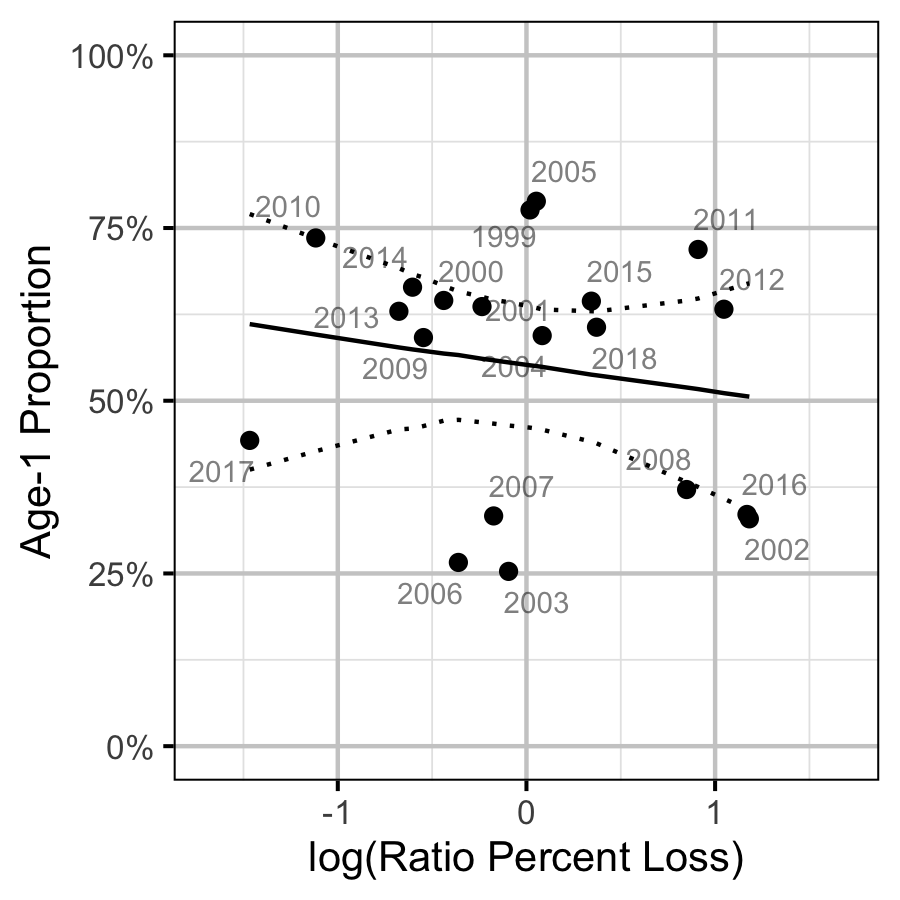
Figure 80. Proportion of Age-1 Mountain Whitefish by percentage egg loss ratio, labelled by spawn year. The predicted relationship is indicated by the solid black line (with 95% CRIs).
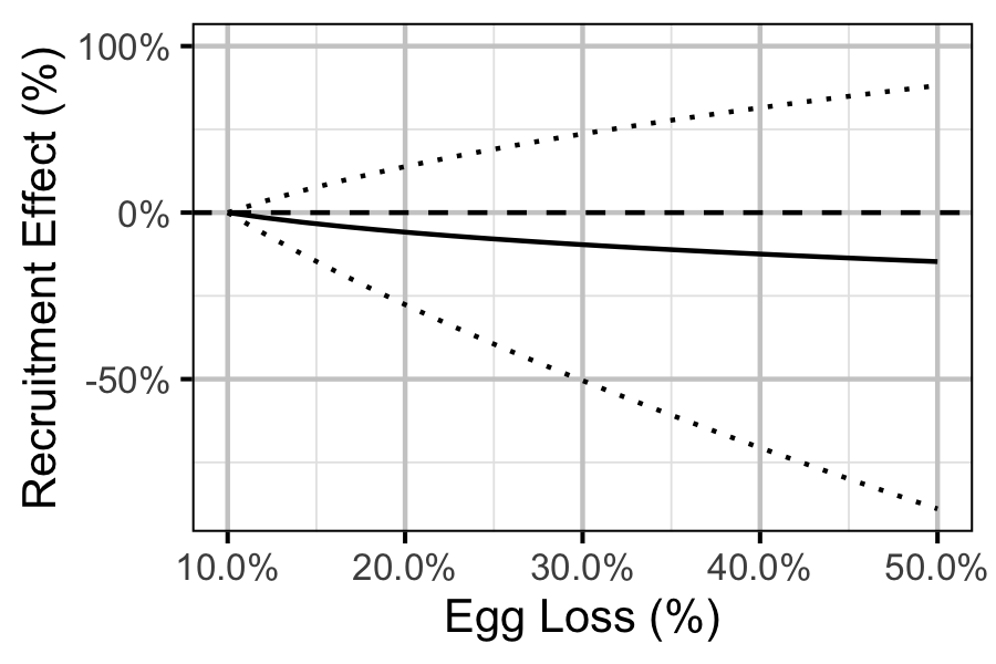
Figure 81. Predicted effect of egg loss on the number of age-1 recruits by egg loss relative to 10% egg loss (with 95% CRIs).
Recommendations
- Develop fecundity vs weight relationship for Mountain Whitefish and Rainbow Trout on the Lower Columbia River.
Acknowledgements
The organisations and individuals whose contributions have made this analysis report possible include:
- BC Hydro
- Okanagan Nation Alliance
- Dave DeRosa
- Amy Duncan
- Golder Associates
- David Roscoe
- Dustin Ford
- Sima Usvyatsov
- Dana Schmidt
- Demitria Burgoon