Lower Columbia River Fish Population Indexing Analysis 2016
The suggested citation for this analytic report is:
Thorley, J.L. and Muir, C.D. (2017) Lower Columbia River Fish Population Indexing Analysis 2016. A Poisson Consulting Analysis Report. URL: https://www.poissonconsulting.ca/f/589633601.
Background
In the mid 1990s BC Hydro began operating Hugh L. Keenleyside (HLK) Dam to reduce dewatering of Mountain Whitefish and Rainbow Trout eggs.
The primary goal of the Lower Columbia River Fish Population Indexing program is to answer two key management questions:
What are the abundance, growth rate, survival rate, body condition, age distribution, and spatial distribution of subadult and adult Whitefish, Rainbow Trout, and Walleye in the Lower Columbia River?
What is the effect of inter-annual variability in the Whitefish and Rainbow Trout flow regimes on the abundance, growth rate, survival rate, body condition, and spatial distribution of subadult and adult Whitefish, Rainbow Trout, and Walleye in the Lower Columbia River?
The inter-annual variability in the Whitefish and Rainbow Trout flow regimes was quantified in terms of the percent egg dewatering as greater flow variability is associated with more egg stranding.
Methods
Data Preparation
The fish indexing data were provided by Okanagan Nation Alliance and Golder Associates in the form of an Access database. The discharge and temperature data were queried from a BC Hydro database maintained by Poisson Consulting. The Rainbow Trout egg dewatering estimates were provided by CLBMON-46 (Irvine, Baxter, and Thorley 2015) and the Mountain Whitefish egg stranding estimates by Golder Associates (2013).
The data were prepared for analysis using R version 3.4.0 (R Core Team 2017).
Data Analysis
Hierarchical Bayesian models were fitted to the data using R version
3.4.0 (R Core Team 2017) and JAGS 4.2.0 (Plummer 2015) which
interfaced with each other via the jmbr package. For additional
information on hierarchical Bayesian modelling in the BUGS language, of
which JAGS uses a dialect, the reader is referred to Kery and Schaub (2011, 41–44).
The one exception was the length-at-age analysis which used a
maximum-likelihood (ML) model which was fitted to the data using TMB
which interfaced with R via the tmbr package. An ML model was used
because the equivalent Bayesian model was becoming prohibitively slow.
Unless indicated otherwise, the models used prior distributions that were vague in the sense that they did not affect the posterior distributions (Kery and Schaub 2011, 36). The posterior distributions were estimated from 2,000 Markov Chain Monte Carlo (MCMC) samples thinned from the second halves of three chains (Kery and Schaub 2011, 38–40). Model convergence was confirmed by ensuring that \(\hat{R} < 1.1\) (Kery and Schaub 2011, 40) for each of the monitored parameters in the model(Kery and Schaub 2011, 61). Where relevant, model adequacy was confirmed by examination of residual plots.
The posterior distributions of the fixed (Kery and Schaub 2011, 75) parameters are summarised in terms of the point estimate, standard deviation (sd), the z-score, lower and upper 95% confidence/credible limits (CLs) and the p-value (Kery and Schaub 2011, 37, 42). The estimate is the median (50th percentile) of the MCMC samples, the z-score is \(\mathrm{mean}/\mathrm{sd}\) and the 95% CLs are the 2.5th and 97.5th percentiles. A p-value of 0.05 indicates that the lower or upper 95% CL is 0.
Variable selection was achieved by dropping fixed (Kery and Schaub 2011, 77–82) variables with two-sided p-values \(\geq\) 0.05 (Kery and Schaub 2011, 37, 42) and random variables with percent relative errors \(\geq\) 80%.
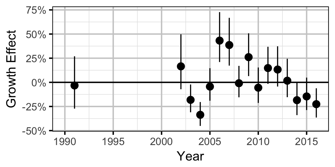
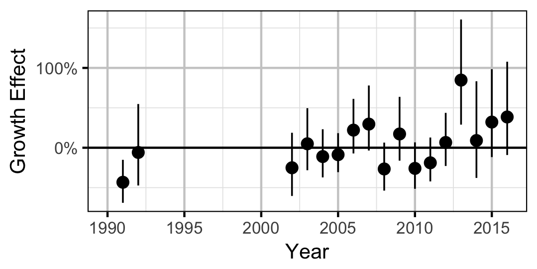
The results are displayed graphically by plotting the modeled relationships between particular variables and the response with 95% credible intervals (CIs) with the remaining variables held constant. In general, continuous and discrete fixed variables are held constant at their mean and first level values respectively while random variables are held constant at their typical values (expected values of the underlying hyperdistributions) (Kery and Schaub 2011, 77–82). Where informative the influence of particular variables is expressed in terms of the effect size (i.e., percent change in the response variable) with 95% CIs (Bradford, Korman, and Higgins 2005).
Model Descriptions
Condition
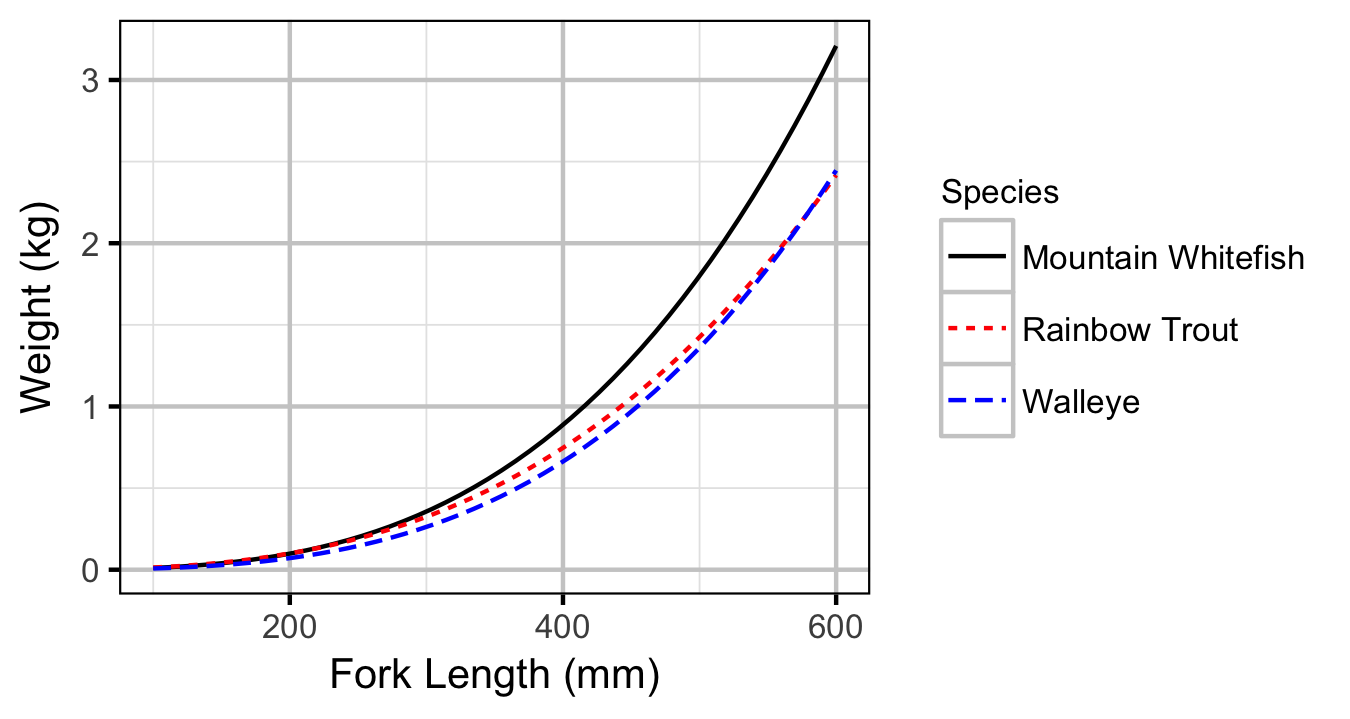
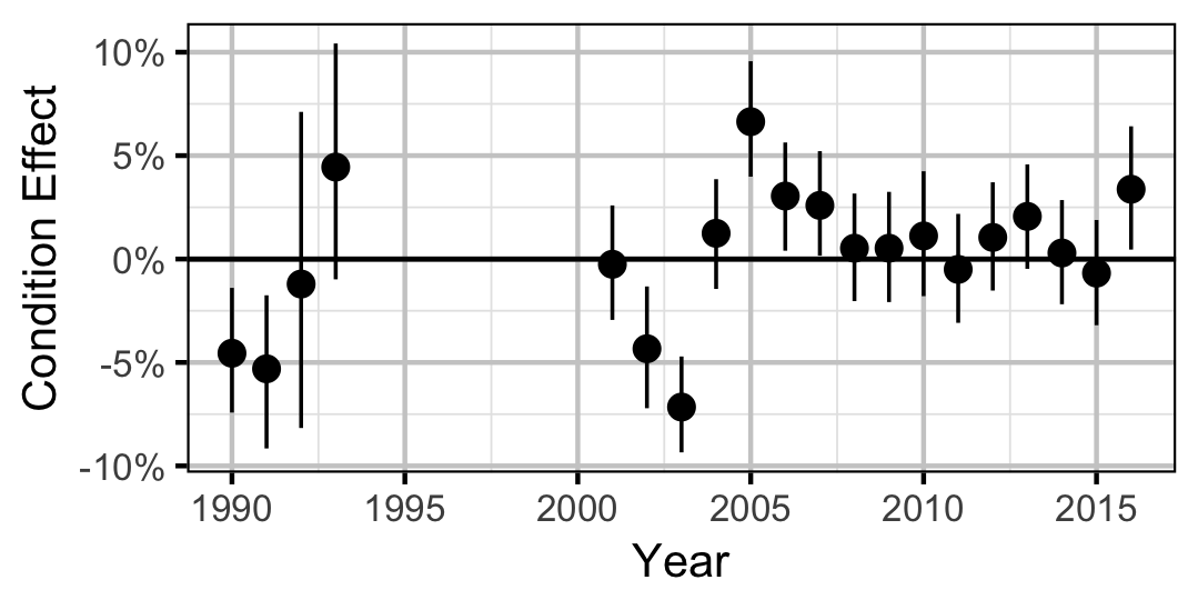
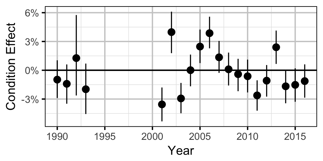
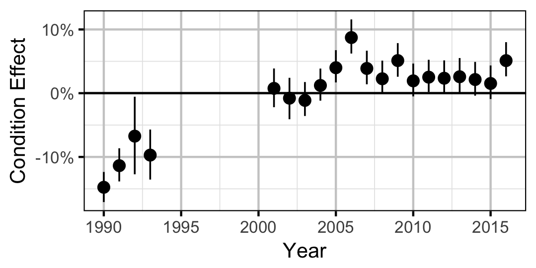
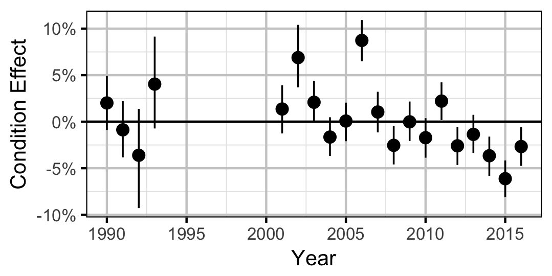
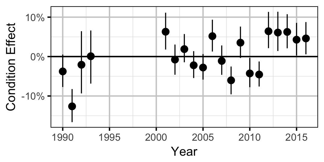
The expected weight of fish of a given length were estimated from the data using a mass-length model (He et al. 2008). Key assumptions of the condition model include:
- The expected weight is allowed to vary with length and date.
- The expected weight is allowed to vary randomly with year.
- The relationship between weight and length is allowed to vary with date.
- The relationship between weight and length is allowed to vary randomly with year.
- The residual variation in weight is log-normally distributed.
Only previously untagged fish were included in models to avoid potential effects of tagging on body condition. Preliminary analyses indicated that the annual variation in weight was not correlated with the annual variation in the relationship between weight and length.
Growth
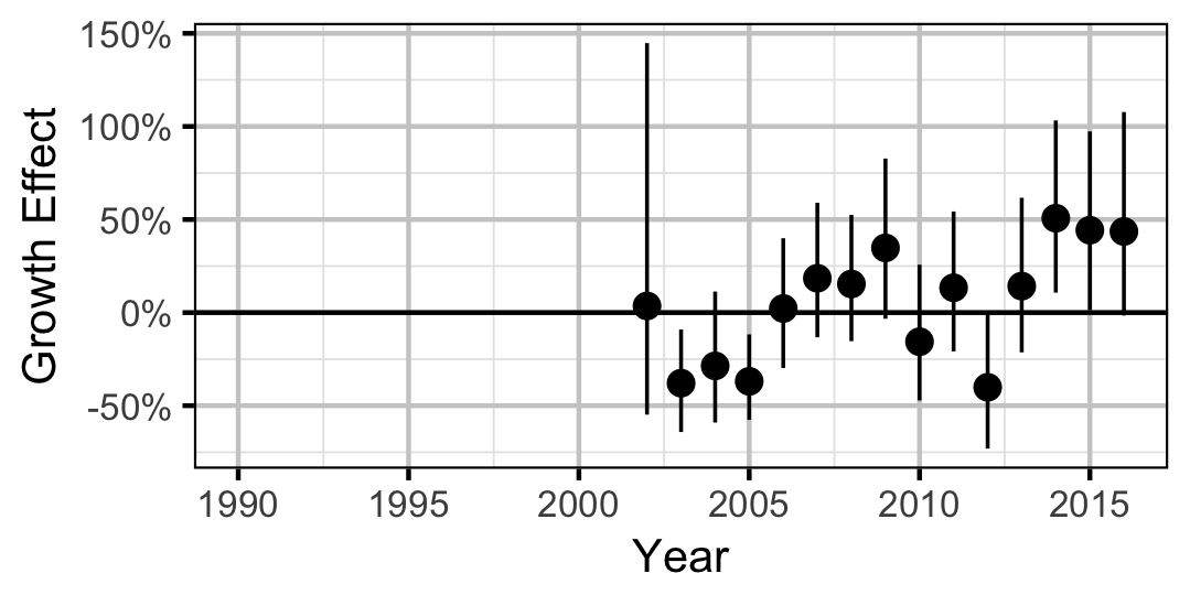
Annual growth of fish were estimated from the inter-annual recaptures using the Fabens method (Fabens 1965) for estimating the von Bertalanffy growth curve (von Bertalanffy 1938). This curve is based on the premise that:
\[ \frac{\text{d}L}{\text{d}t} = k (L_{\infty} - L)\]
where \(L\) is the length of the individual, \(k\) is the growth coefficient and \(L_{\infty}\) is the maximum length.
Integrating the above equation gives:
\[ L_t = L_{\infty} (1 - e^{-k(t - t_0)})\]
where \(L_t\) is the length at time \(t\) and \(t_0\) is the time at which the individual would have had zero length.
The Fabens form allows
\[ L_r = L_c + (L_{\infty} - L_c) (1 - e^{-kT})\]
where \(L_r\) is the length at recapture, \(L_c\) is the length at capture and \(T\) is the time between capture and recapture.
Key assumptions of the growth model include:
- The mean maximum length \(L_{\infty}\) is constant.
- The growth coefficient \(k\) is allowed to vary randomly with year.
- The residual variation in growth is normally distributed.
Length-At-Age
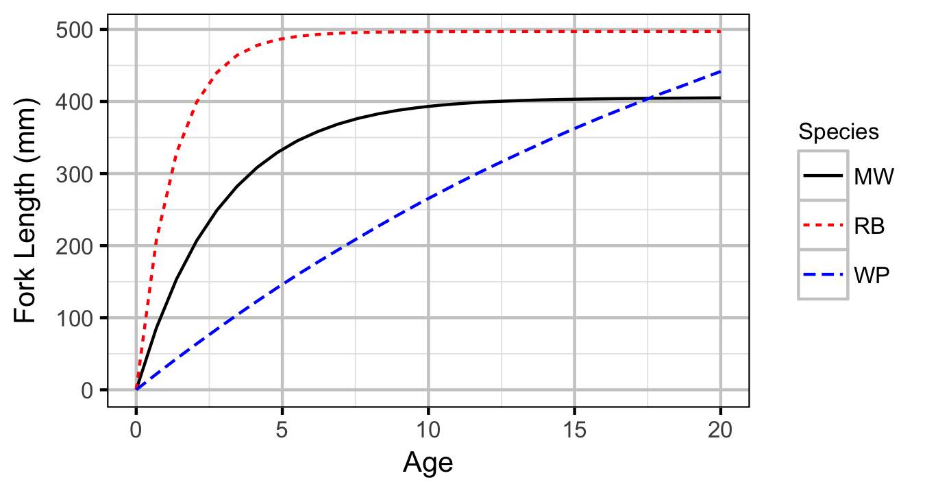
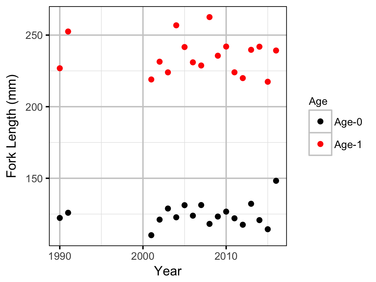
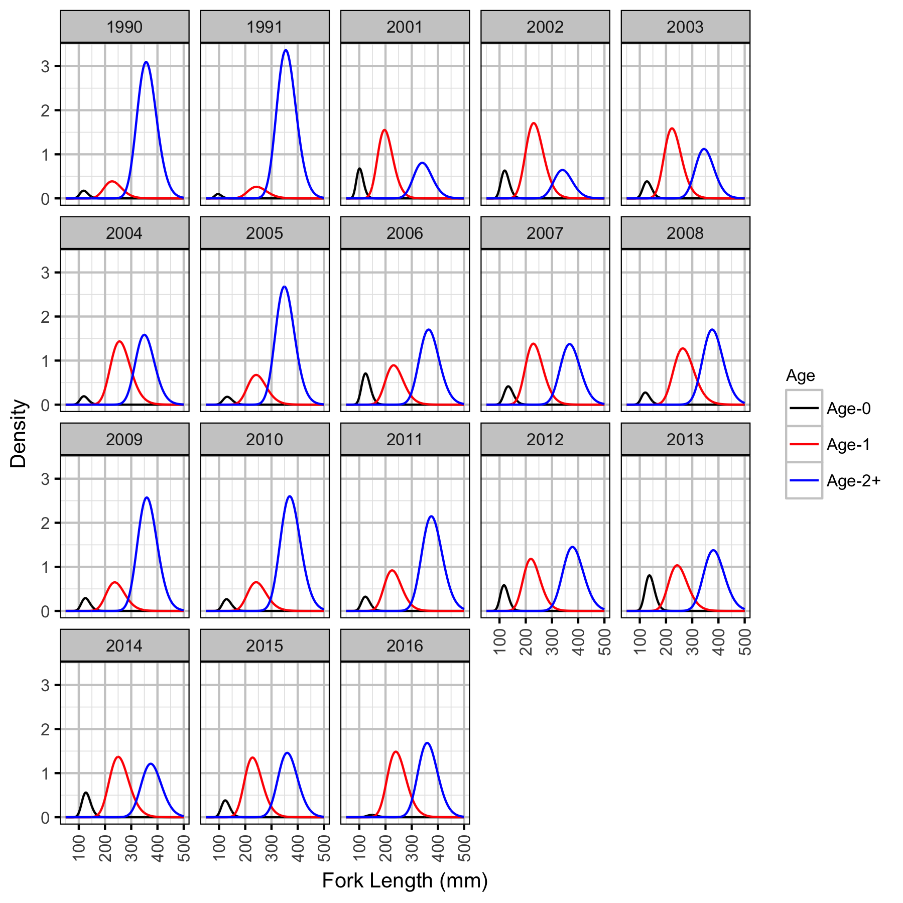
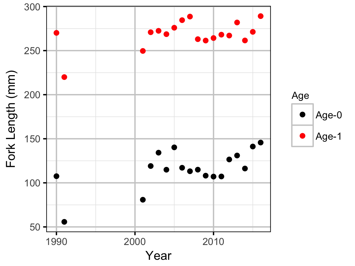
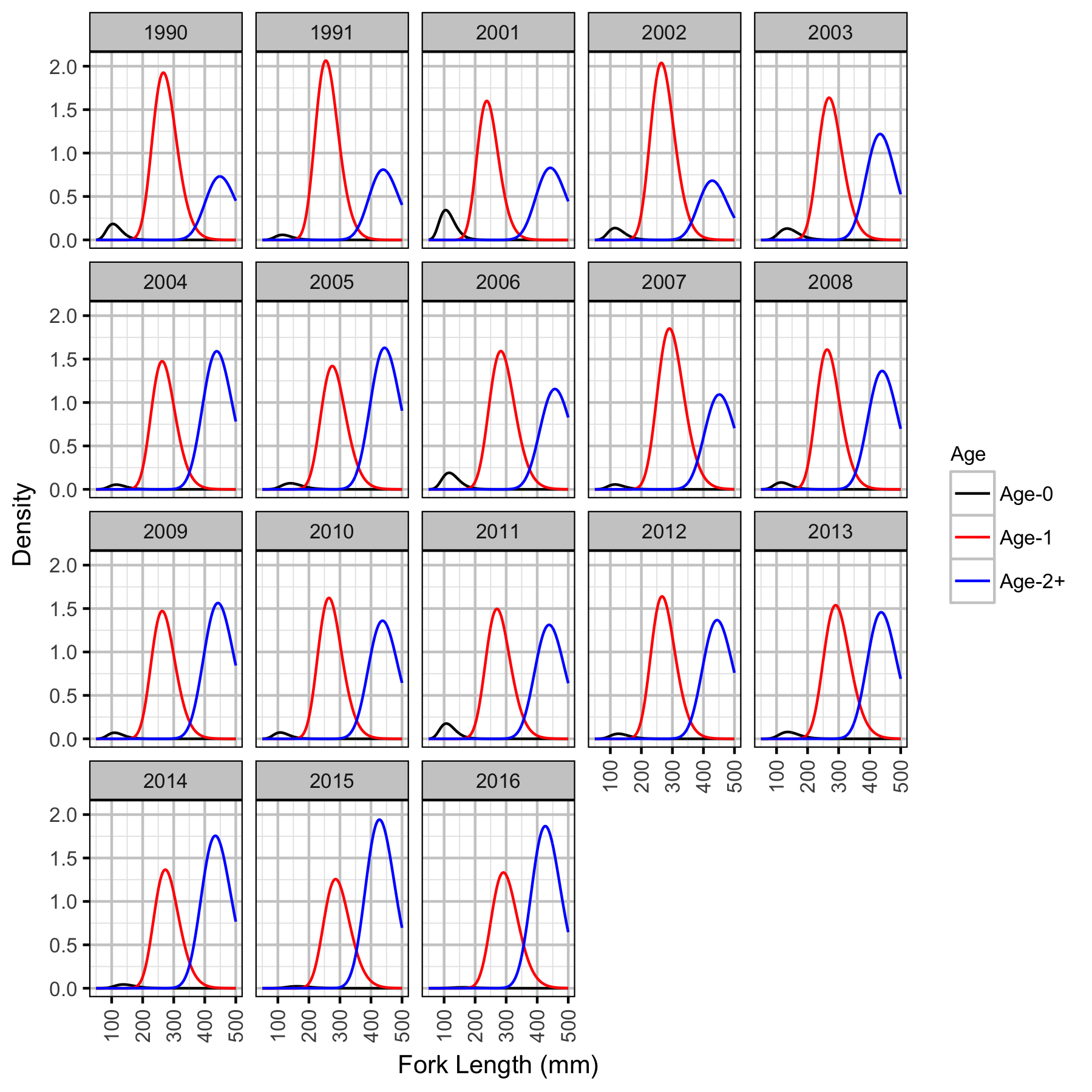
The expected length-at-age of Mountain Whitefish and Rainbow Trout were estimated from annual length-frequency distributions using a finite mixture distribution model (Macdonald and Pitcher 1979). Key assumptions of the length-at-age model include:
- There are three distinguishable age-classes for each species: Age-0, Age-1 and Age-2+.
- The proportion of fish in each age-class is allowed to vary with year.
- The expected length increases with age-class.
- The expected length is allowed to vary with year within age-class.
- The expected length is allowed to vary as a linear function of date.
- The relationship between length and date is allowed to vary with age-class.
- The residual variation in log-tranformed length is normally distributed.
- The standard deviation of this normal distribution varies with age-class.
The model was used to estimate the cutoffs between age-classes by year and date within year to account for growth. For the purposes of estimating other population parameters by age-class, Age-0 individuals were classified as fry, Age-1 individuals were classified as subadult, and Age-2+ individuals were classified as adult. Walleye could not be separated by life stage due to a lack of discrete modes in the length-frequency distributions for this species. Consequently, all captured Walleye were considered to be adults.
The results include plots of the age-class density for each year by length as predicted by the length-at-age model. Density is a measure of relative frequency for continuous values.
Observer Length Correction
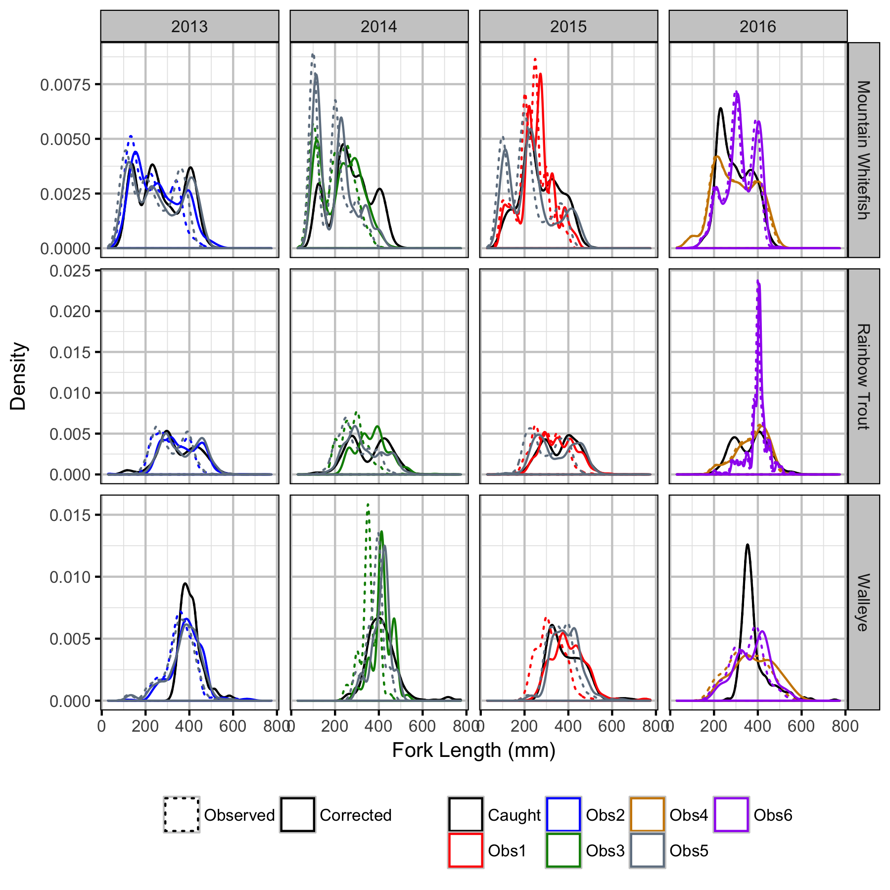
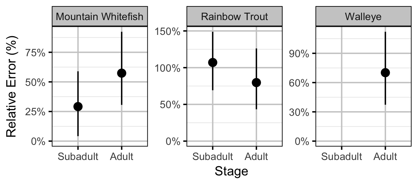
The bias (accuracy) and error (precision) in observer’s fish length estimates were quantified using a model with a categorical distribution which compared the proportions of fish in different length-classes for each observer to the equivalent proportions for the measured fish. Key assumptions of the observer length correction model include:
- The proportion of fish in each length-class is allowed to vary with year.
- The expected length bias is allowed to vary with observer.
- The expected length error is allowed to vary with observer.
- The expected length bias and error for a given observer does not vary by year.
- The residual variation in length is normally distributed.
The observed fish lengths were corrected for the estimated length biases before being classified as fry, subadult and adult based on the length-at-age cutoffs.
Survival
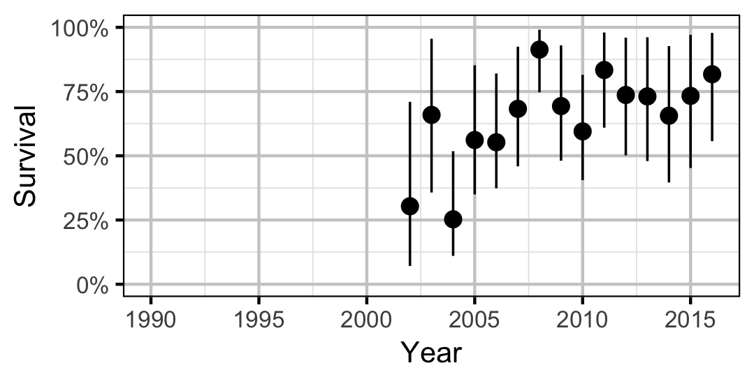
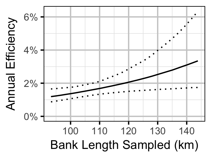
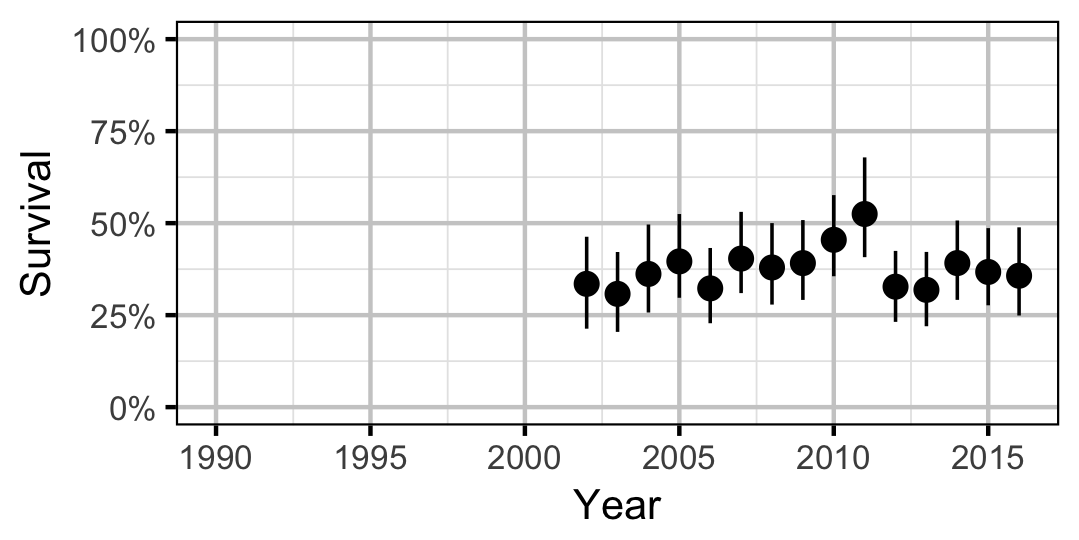
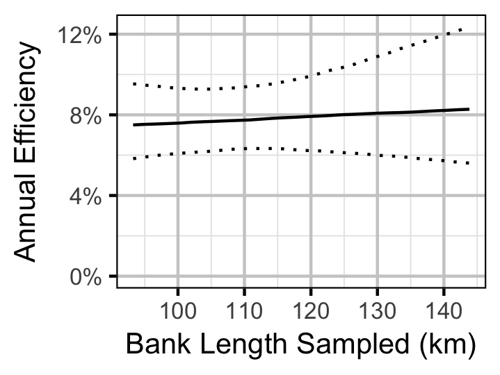
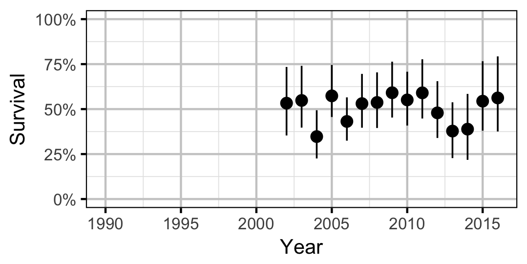
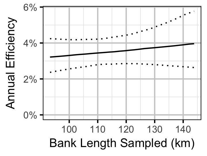
The annual adult survival rate was estimated by fitting a Cormack-Jolly-Seber model (Kery and Schaub 2011, 220–31) to inter-annual recaptures of adults.
Key assumptions of the survival model include:
- Survival varies randomly with year.
- The encounter probability for adults is allowed to vary with the total bank length sampled.
Site Fidelity
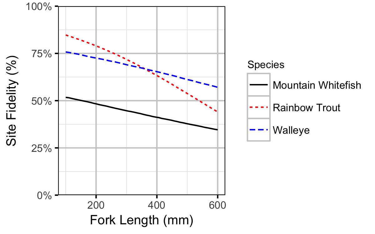
The extent to which sites are closed, i.e., fish remain at the same site between sessions, was evaluated with a logistic ANCOVA (Kery 2010). The model estimates the probability that intra-annual recaptures were caught at the same site versus a different one. Key assumptions of the site fidelity model include:
- The expected site fidelity is allowed to vary with fish length.
- Observed site fidelity is Bernoulli distributed.
Length as a second-order polynomial was not found to be a significant predictor for site fidelity.
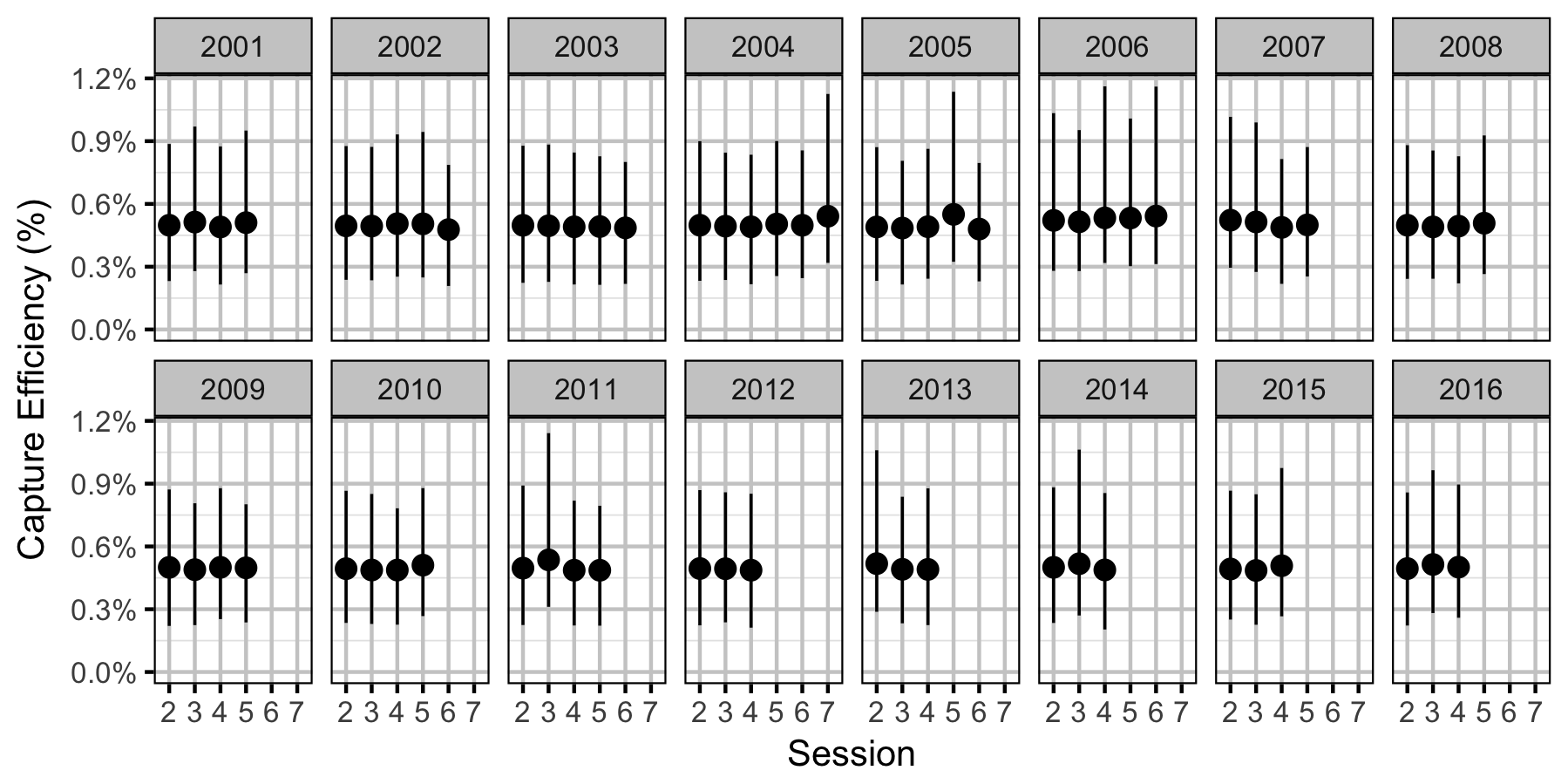
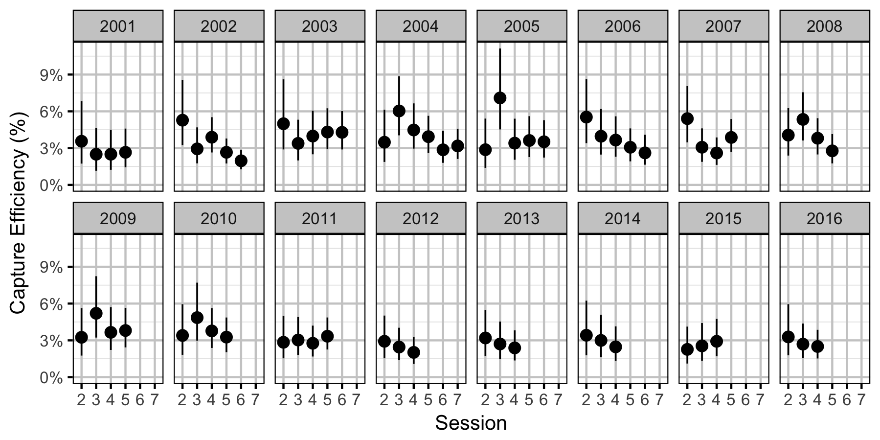
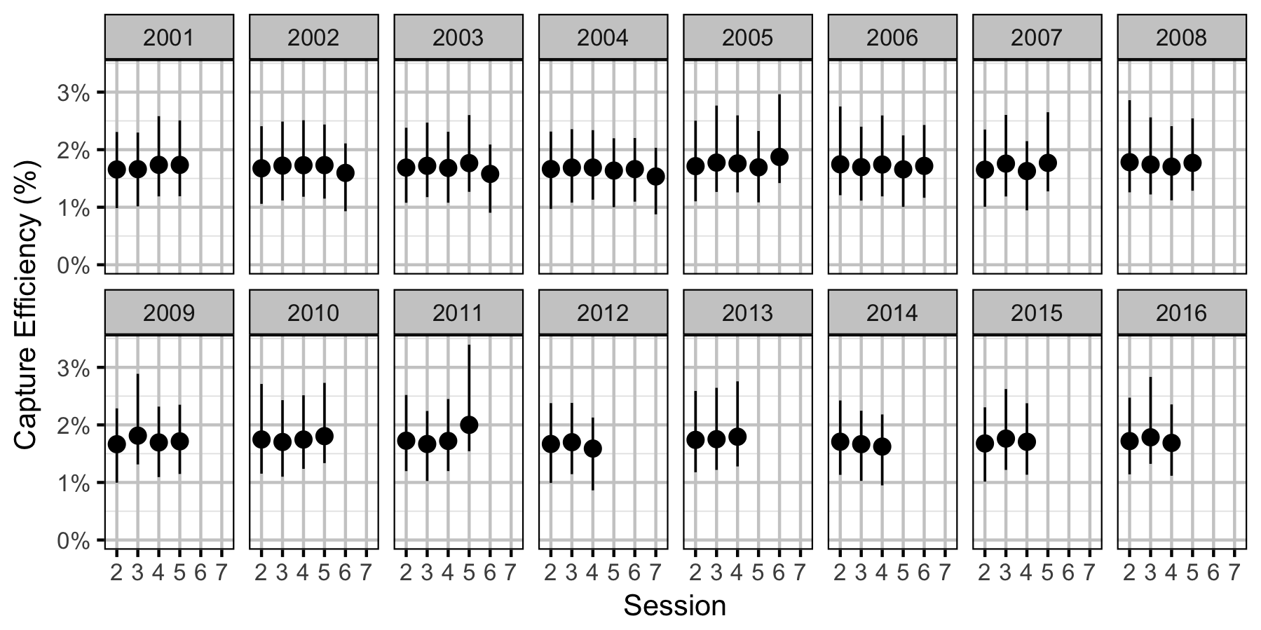
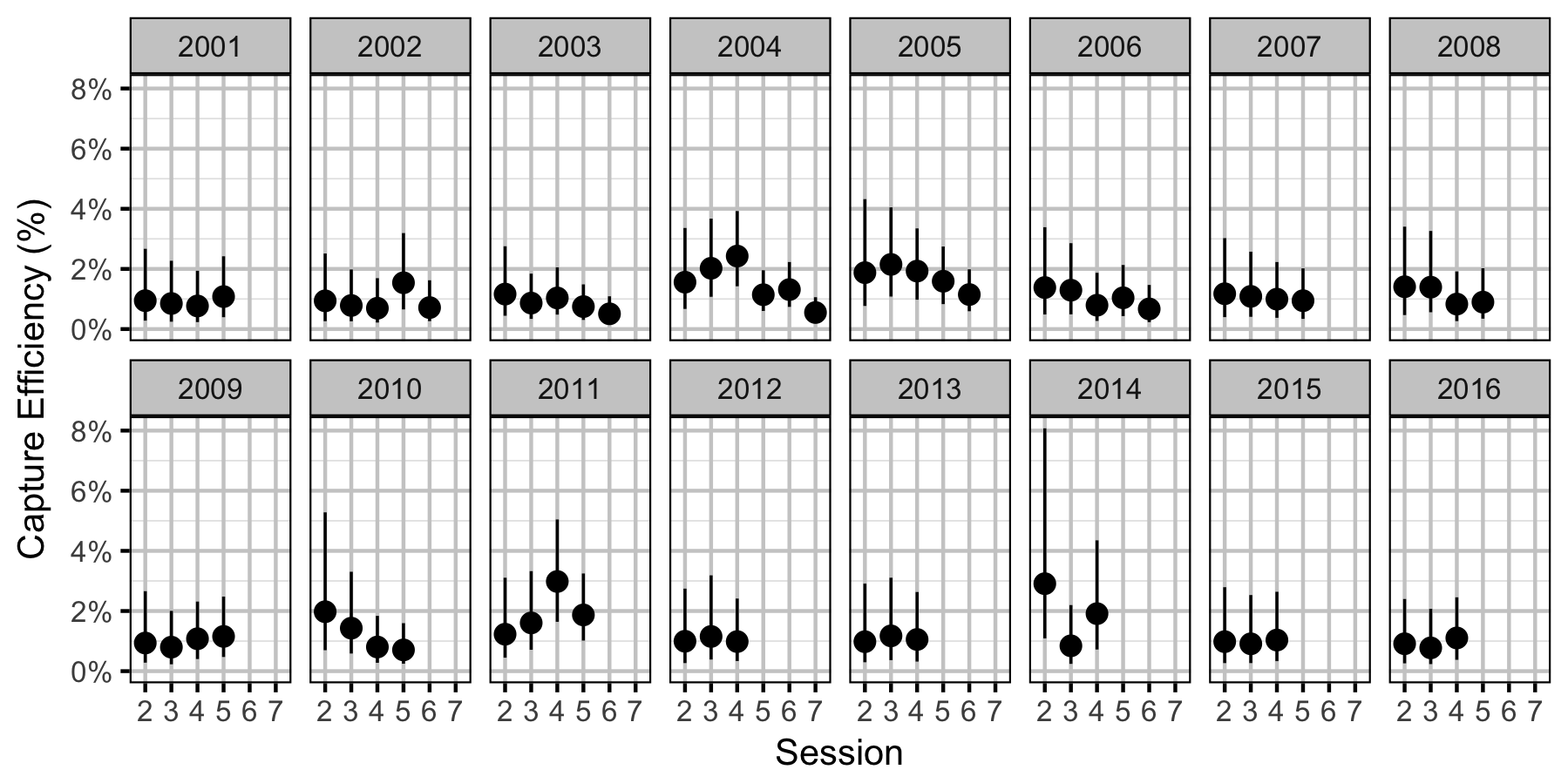
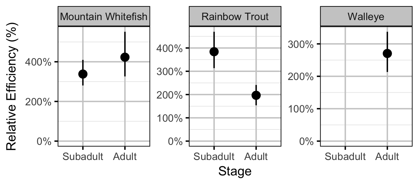
Capture Efficiency
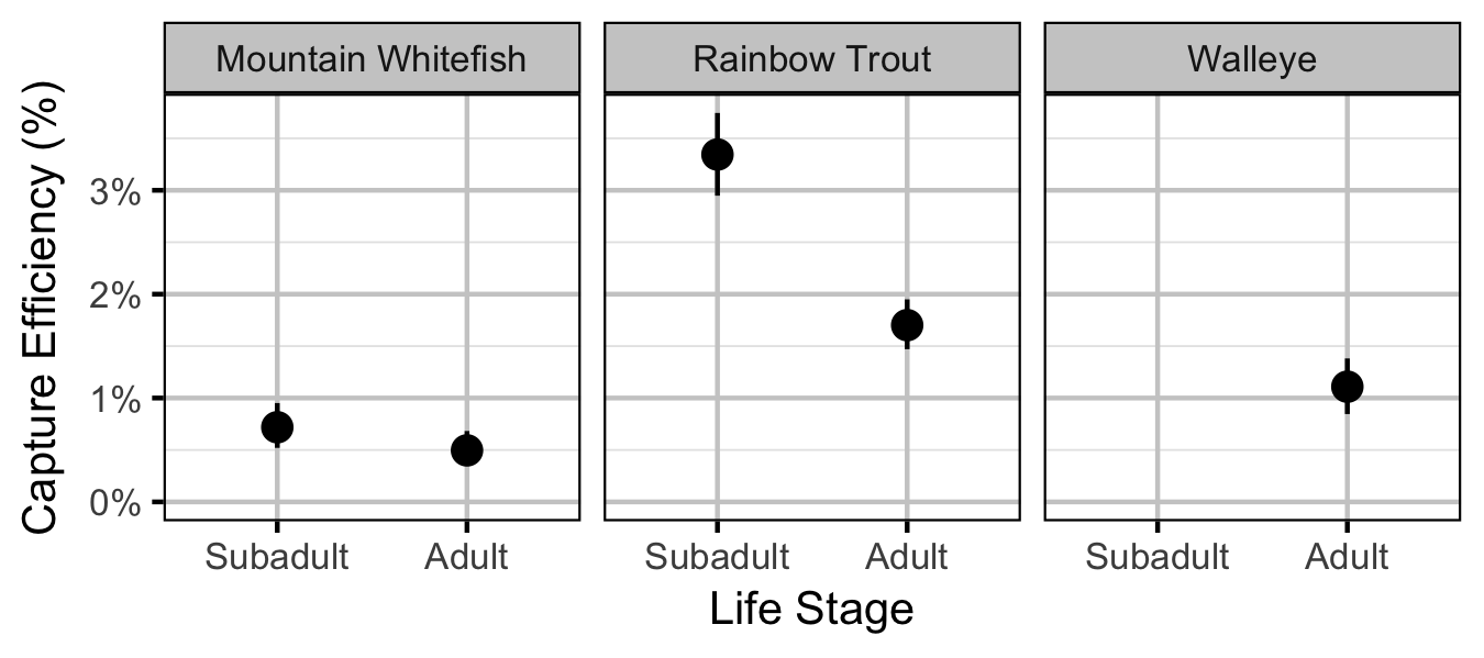
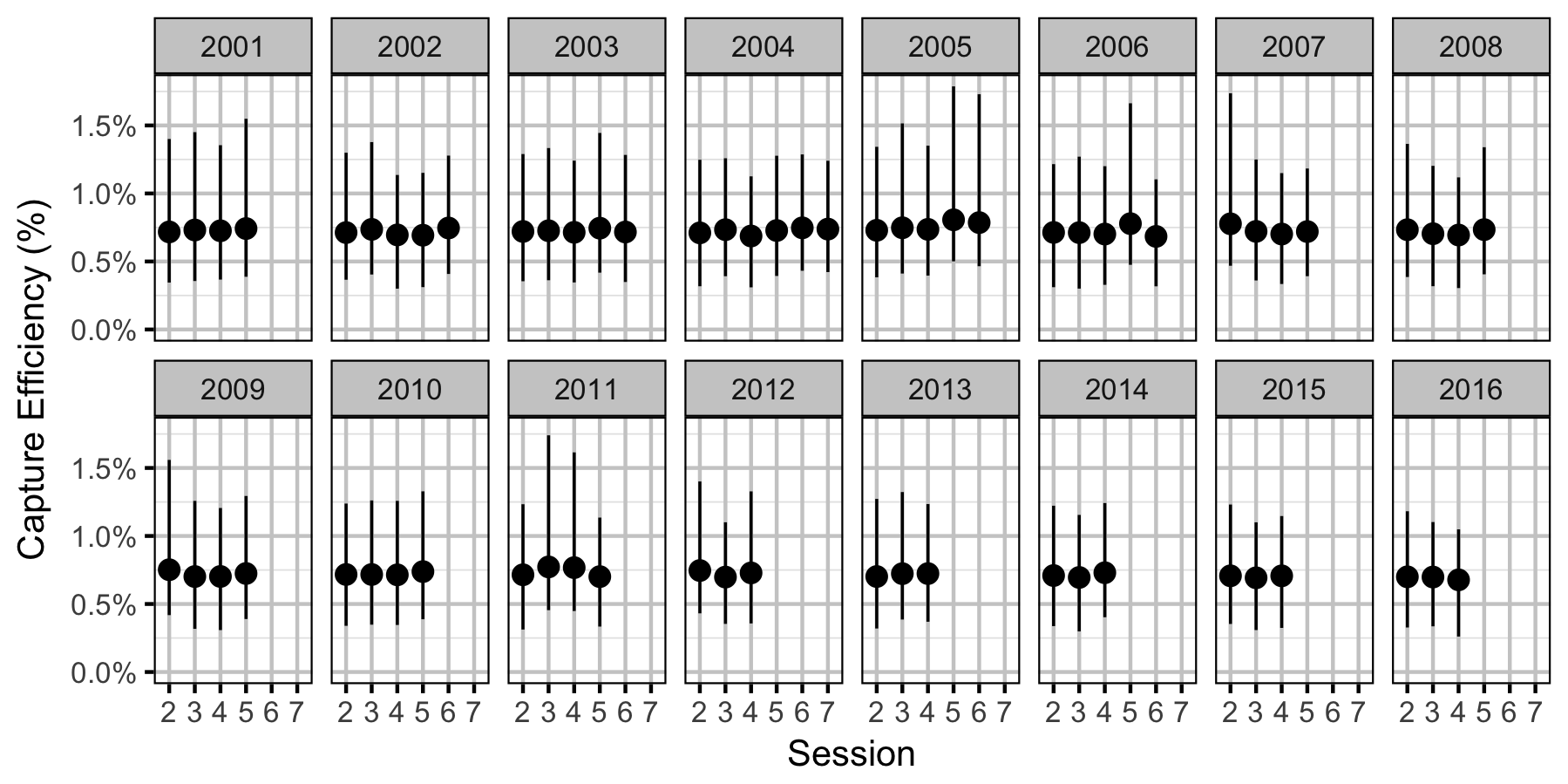
The probability of capture was estimated using a recapture-based binomial model (Kery and Schaub 2011, 134–36, 384–88).
Key assumptions of the capture efficiency model include:
- The capture probability varies randomly by session within year.
- The probability of a marked fish remaining at a site is the estimated site fidelity.
- The number of recaptures is described by a binomial distribution.
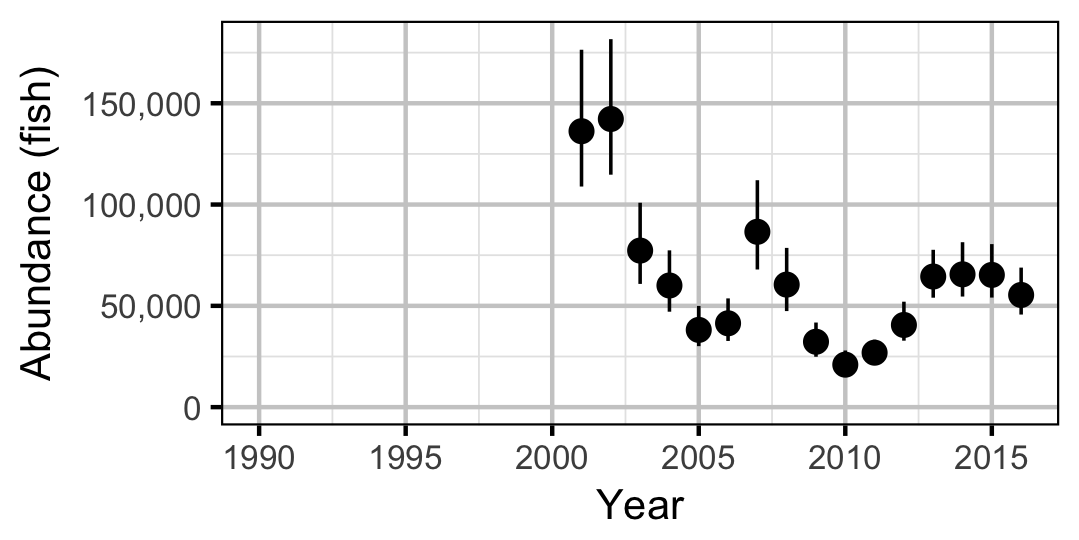
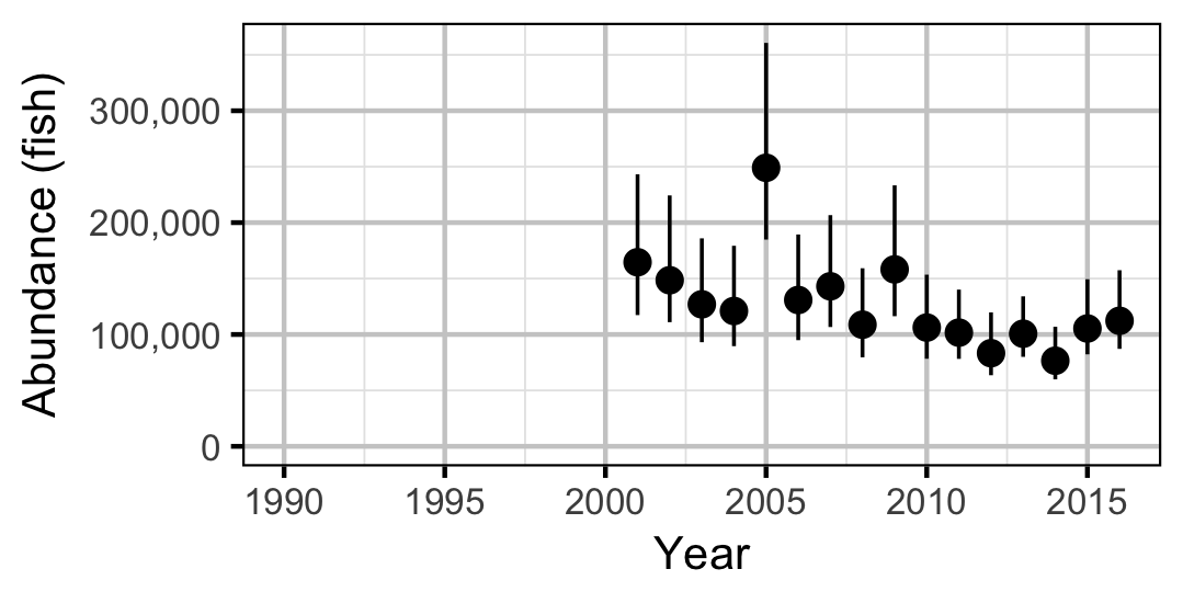
Abundance
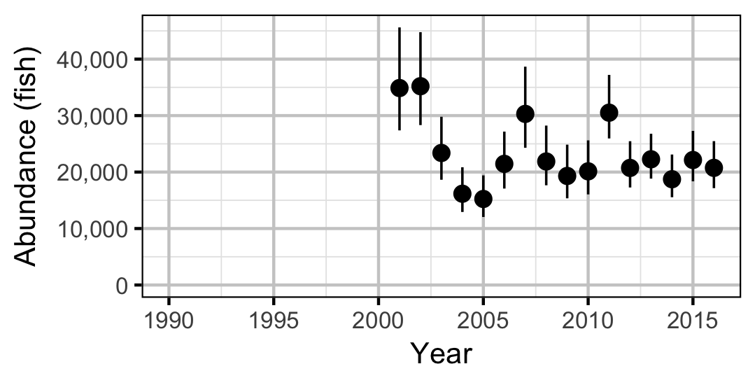
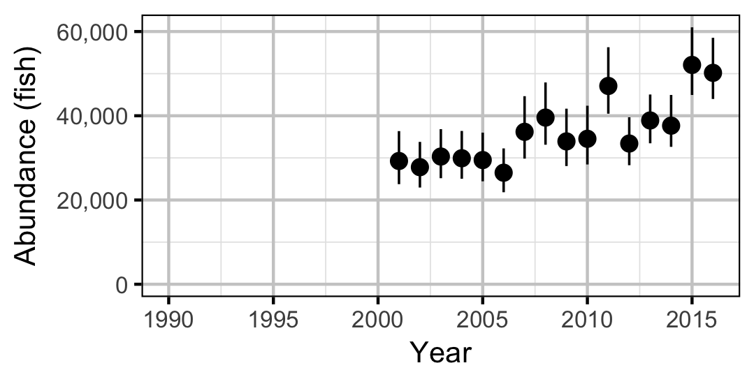
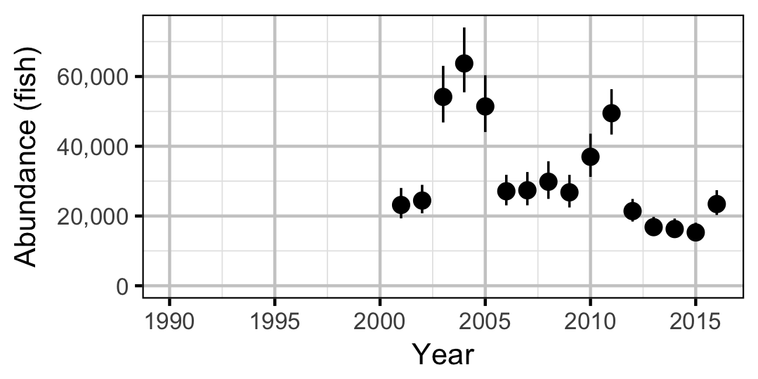
The abundance was estimated from the catch and bias-corrected observer count data using an overdispersed Poisson model (Kery and Schaub 2011, 55–56).
Key assumptions of the abundance model include:
- The capture efficiency is the point estimate from the capture efficiency model.
- The efficiency varies by visit type (catch or count).
- The lineal fish density varies randomly with site, year and site within year.
- The overdispersion varies by visit type (count or catch).
- The catches and counts are described by a gamma-Poisson distribution.
Stock-Recruitment
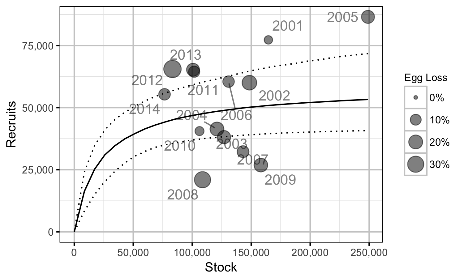
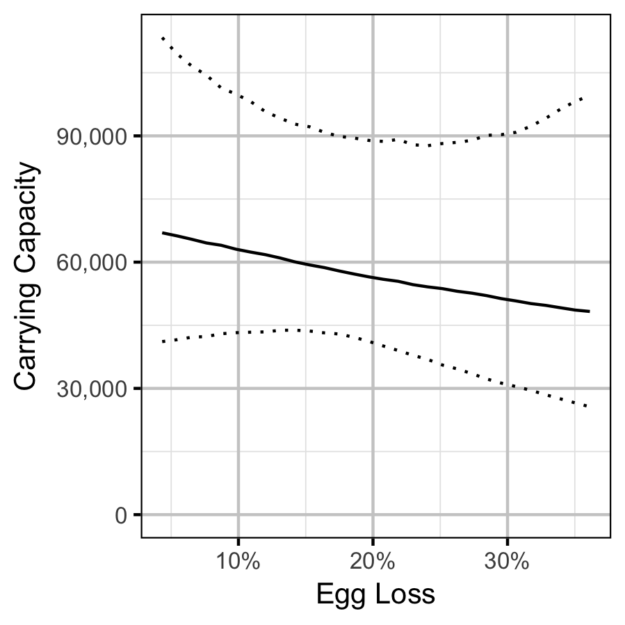
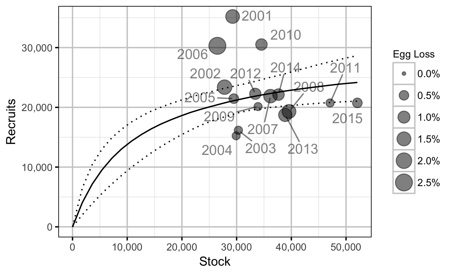
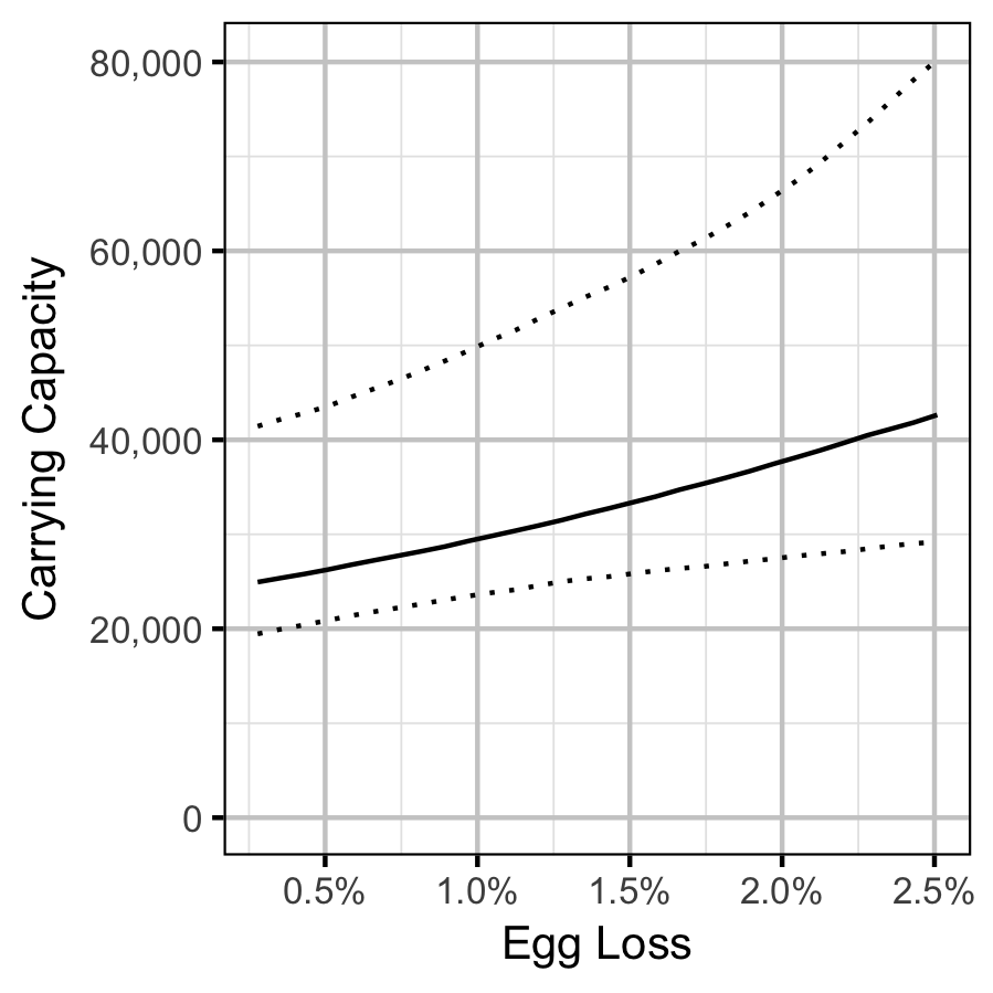
The relationship between the adults and the resultant number of age-1 subadults was estimated using a Beverton-Holt stock-recruitment model (Walters and Martell 2004):
\[ R = \frac{\alpha \cdot S}{1 + \beta \cdot S} \quad,\]
where \(S\) is the adults (stock), \(R\) is the subadults (recruits), \(\alpha\) is the recruits per spawner at low density and \(\beta\) determines the density-dependence.
Key assumptions of the stock-recruitment model include:
- The prior for \(\log(\alpha)\) is a truncated normal distribution from \(\log(1)\) to \(\log(5)\).
- The recruits per spawner varies with the proportional egg loss.
- The residual variation in the number of recruits is log-normally distributed.
The carrying capacity \(K\) is given by the relationship:
\[ K = \frac{\alpha}{\beta} \quad.\]
Scale Age
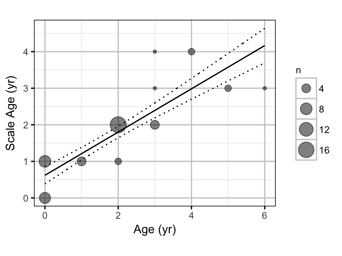
The age of Mountain Whitefish was estimated from scales using an automated algorithm. The algorithm estimates the age of individual fish by finding annuli among the growth circuli in the scale. Specifically, annuli represent blocks of slow growth – short inter-circuli distance – during the winter. The algorithm takes scale growth between circuli, calculates a moving average growth rate, and then calculates a moving average of the rate of change in growth. For brevity, we refer to the “rate of change in growth” as “dGrowth”.Periods of rapid deceleration (dGrowth < 0) correspond to winter and mark an annulus. Specifically, we defined an annulus as a run of negative dGrowth values. Because of noise in the measurements, these runs had to be of a minimum length. We estimated the window size for calculating moving averages and this minimum length by tuning the algorithm to most accurately predict scale ages from recaptured fish of known age. During tuning, we found that a window size of seven circuli was best for calculating the moving average growth rate; a window size of 17 circuli was best for calculating dGrowth. Note that a larger window size leads to greater smoothing in the series. We estimated the minimum length for a run to be four. Once the algorithm was tuned, we applied to fish scales of unknown age.
Key assumptions of the scale age algorithm include:
- Growth decelerates in the fall/winter and accelerates in spring/summer
- The actual age is the year of capture minus the hatch year
- The scale age varies linearly with age.
Age-Ratios
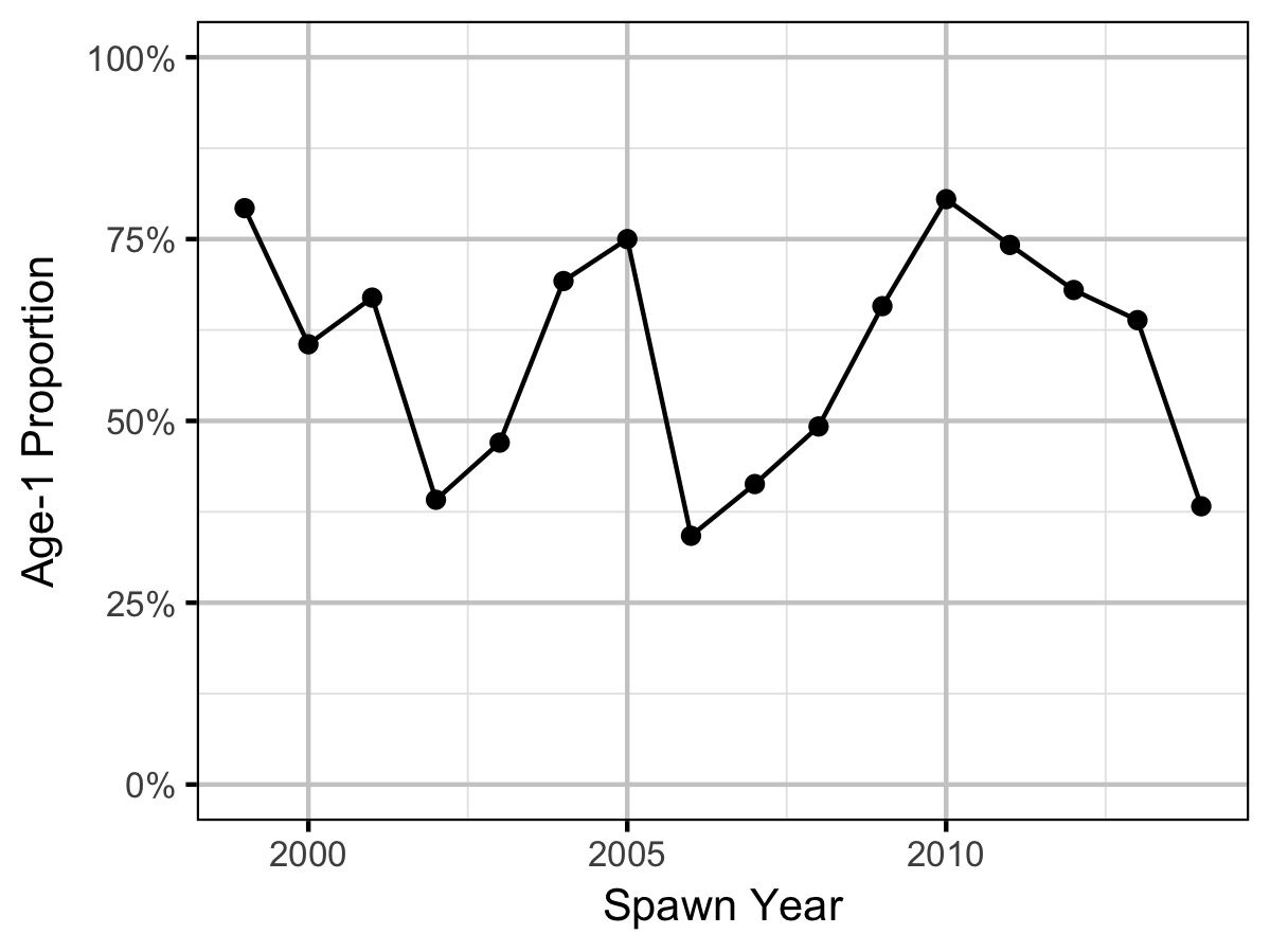
The proportion of Age-1 Mountain Whitefish \(r^1_t\) from a given spawn year \(t\) is calculated from the number of Age-1 & Age-2 fish \(N^1_t\) & \(N^2_t\) respectively, which were lead or lagged so that all values were with respect to the spawn year:
\[r^1_t = \frac{N^1_{t+2}}{N^1_{t+2} + N^2_{t+2}}\]
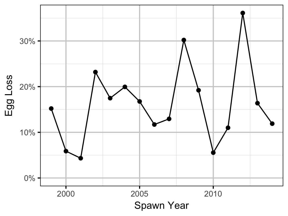
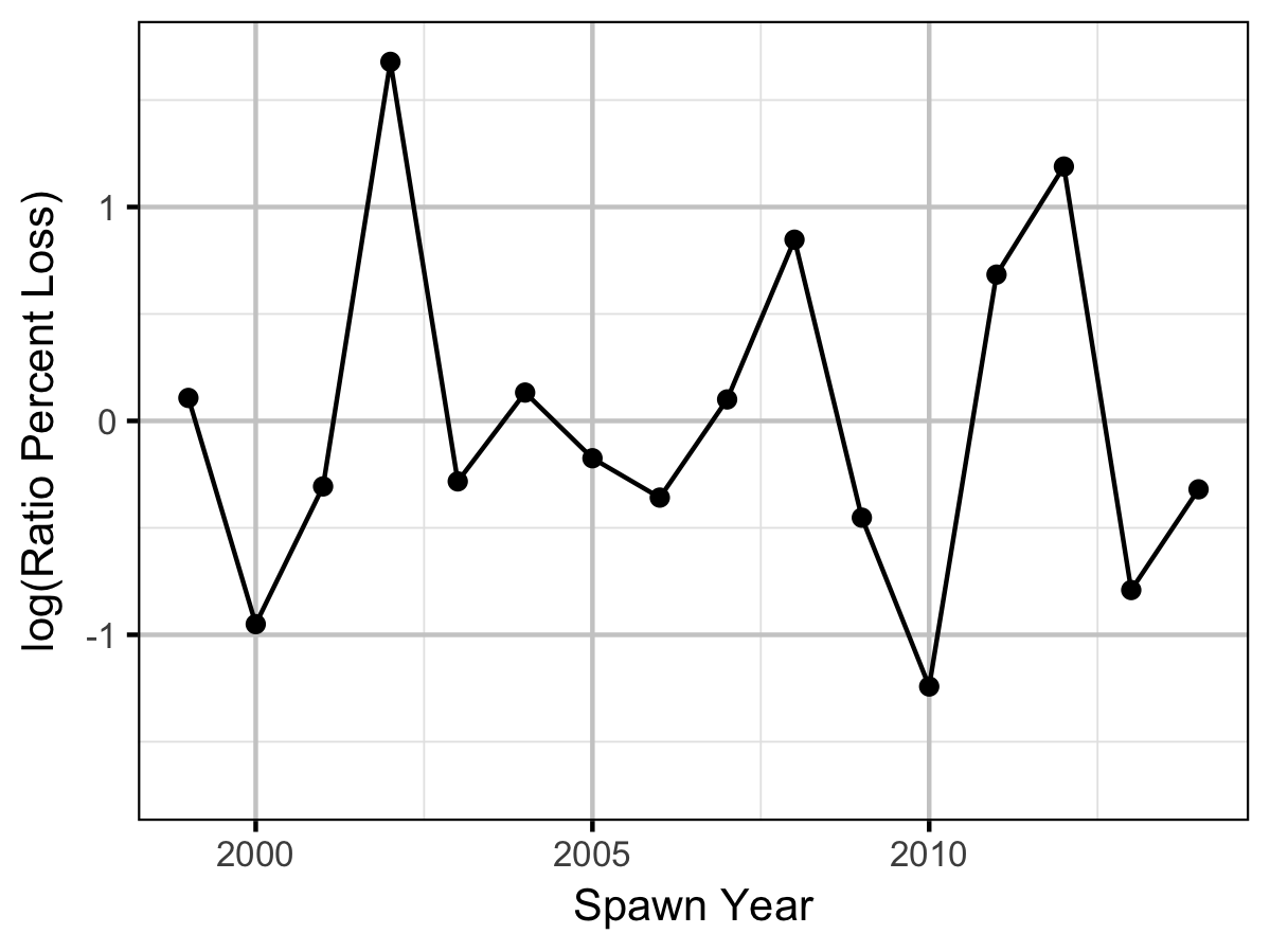
As the number of Age-2 fish might be expected to be influenced by the percentage egg loss \(Q_t\) three years prior, the predictor variable \(\Pi_t\) used is:
\[\Pi_t = \textrm{log}(Q_t/Q_{t-1})\]
The ratio was logged to ensure it was symmetrical about zero (Tornqvist, Vartia, and Vartia 1985).
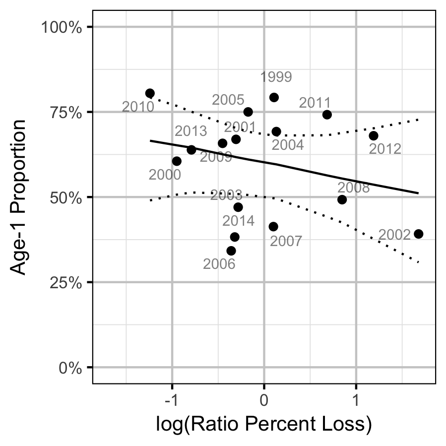
The relationship between \(r^1_t\) and \(\Pi_t\) was estimated using a hierarchical Bayesian logistic regression (Kery 2010) loss model.
Key assumptions of the final model include:
- The log odds of the proportion of Age-1 fish varies linearly with the log of the ratio of the percent egg losses.
- The numbers of Age-1 fish are extra-Binomially distributed.
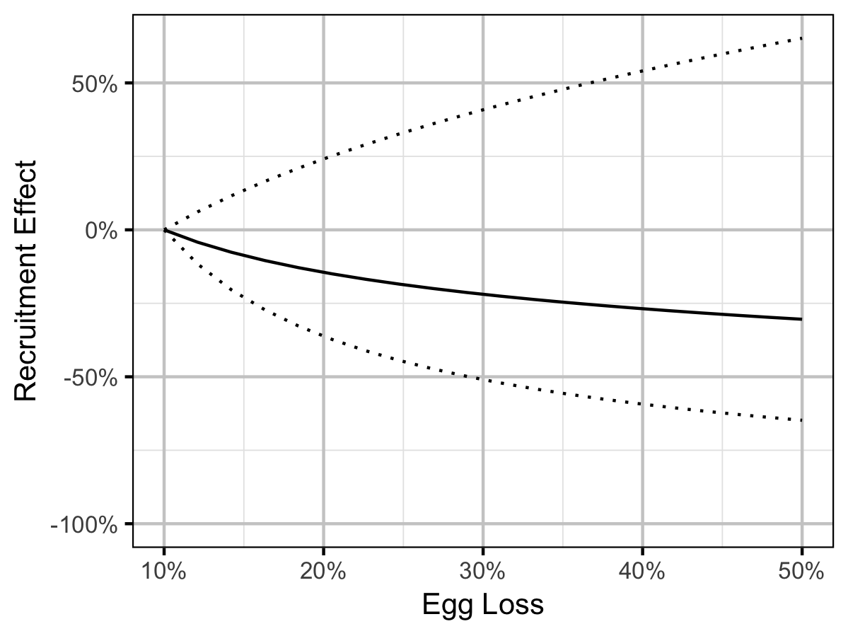
The relationship between percent dewatering and subsequent recruitment is expected to depend on stock abundance (Subbey et al. 2014) which might be changing over the course of the study. Consequently, preliminary analyses allowed the slope of the regression line to change by year. However, year was not a significant predictor and was therefore removed from the final model. The effect of dewatering on Mountain Whitefish abundance was expressed in terms of the predicted percent change in Age-1 Mountain Whitefish abundance by egg loss in the spawn year relative to 10% egg loss in the spawn year. The egg loss in the previous year was fixed at 10%. The percent change could not be calculated relative to 0% in the spawn or previous year as \(\Pi_t\) is undefined in either case.
Model Templates
Condition
model {
  bWeight ~ dnorm(5, 5^-2)
  bWeightLength ~ dnorm(3, 2^-2)

  bWeightDayte ~ dnorm(0, 2^-2)
  bWeightLengthDayte ~ dnorm(0, 2^-2)

  sWeightYear ~ dnorm(0, 2^-2)
  sWeightLengthYear ~ dnorm(0, 2^-2)
  for (i in 1:nYear) {
    bWeightYear[i] ~ dnorm(0, exp(sWeightYear)^-2)
    bWeightLengthYear[i] ~ dnorm(0, exp(sWeightLengthYear)^-2)
  }

  sWeight ~ dnorm(0, 5^-2)
  for(i in 1:length(Length)) {
    log(eWeight[i]) <- bWeight +
                        bWeightDayte * Dayte[i] +
                        bWeightYear[Year[i]] +
                        (bWeightLength +
                          bWeightLengthDayte * Dayte[i] +
                          bWeightLengthYear[Year[i]]) * Length[i]

    Weight[i] ~ dlnorm(log(eWeight[i]), exp(sWeight)^-2)
  }
..
Template 1.
Growth
model {
  bK ~ dnorm (0, 5^-2)
  sKYear ~ dnorm(0, 5^-2)

  for (i in 1:nYear) {
    bKYear[i] ~ dnorm(0, exp(sKYear)^-2)
    log(eK[i]) <- bK + bKYear[i]
  }

  bLinf ~ dunif(100, 1000)
  sGrowth ~ dnorm(0, 5^-2)
  for (i in 1:length(Year)) {
    eGrowth[i] <- (bLinf - LengthAtRelease[i]) * (1 - exp(-sum(eK[Year[i]:(Year[i] + dYears[i] - 1)])))
    Growth[i] ~ dnorm(eGrowth[i], exp(sGrowth)^-2)
  }
..
Template 2.
Observer Length Correction
model{
  for(j in 1:nAnnual){
    for(i in 1:nClass) {
      dClass[i, j] <- 1
    }
    pClass[1:nClass, j] ~ ddirch(dClass[, j])
  }

  bLength[1] <- 1
  sLength[1] <- 1

  for(i in 2:nObserver) {
    bLength[i] ~ dunif(0.5, 2)
    sLength[i] ~ dunif(2, 10)
  }

  for(i in 1:length(Length)){
    eClass[i] ~ dcat(pClass[, Annual[i]])
    eLength[i] <- bLength[Observer[i]] * ClassLength[eClass[i]]
    eSLength[i] <- sLength[Observer[i]] * ClassSD
    Length[i] ~ dnorm(eLength[i], eSLength[i]^-2)
  }
..
Template 3.
Survival
model{
  bEfficiency ~ dnorm(0, 5^-2)
  bEfficiencySampledLength ~ dnorm(0, 5^-2)

  bSurvival ~ dnorm(0, 5^-2)

  sSurvivalYear ~ dnorm(0, 5^-2)
  for(i in 1:nYear) {
    bSurvivalYear[i] ~ dnorm(0, exp(sSurvivalYear)^-2)
  }

  for(i in 1:(nYear-1)) {
    logit(eEfficiency[i]) <- bEfficiency + bEfficiencySampledLength * SampledLength[i]
    logit(eSurvival[i]) <- bSurvival + bSurvivalYear[i]

    eProbability[i,i] <- eSurvival[i] * eEfficiency[i]
    for(j in (i+1):(nYear-1)) {
      eProbability[i,j] <- prod(eSurvival[i:j]) * prod(1-eEfficiency[i:(j-1)]) * eEfficiency[j]
    }
    for(j in 1:(i-1)) {
      eProbability[i,j] <- 0
    }
  }
  for(i in 1:(nYear-1)) {
    eProbability[i,nYear] <- 1 - sum(eProbability[i,1:(nYear-1)])
  }

  for(i in 1:(nYear - 1)) {
    Marray[i, 1:nYear] ~ dmulti(eProbability[i,], Released[i])
  }
..
Template 4.
Site Fidelity
model {

  bFidelity ~ dnorm(0, 2^-2)
  bLength ~ dnorm(0, 2^-2)

  for (i in 1:length(Fidelity)) {
    logit(eFidelity[i]) <- bFidelity + bLength * Length[i]
    Fidelity[i] ~ dbern(eFidelity[i])
  }
..
Template 5.
Capture Efficiency
model {

  bEfficiency ~ dnorm(0, 5^-2)

  sEfficiencySessionAnnual ~ dnorm(0, 2^-2)
  for (i in 1:nSession) {
    for (j in 1:nAnnual) {
      bEfficiencySessionAnnual[i, j] ~ dnorm(0, exp(sEfficiencySessionAnnual)^-2)
    }
  }

  for (i in 1:length(Recaptures)) {

    logit(eEfficiency[i]) <- bEfficiency + bEfficiencySessionAnnual[Session[i], Annual[i]]

    eFidelity[i] ~ dnorm(Fidelity[i], FidelitySD[i]^-2) T(FidelityLower[i], FidelityUpper[i])
    Recaptures[i] ~ dbin(eEfficiency[i] * eFidelity[i], Tagged[i])
  }
..
Template 6.
Abundance
model {
  bDensity ~ dnorm(5, 5^-2)

  sDensityAnnual ~ dnorm(0, 2^-2)
  for (i in 1:nAnnual) {
    bDensityAnnual[i] ~ dnorm(0, exp(sDensityAnnual)^-2)
  }

  sDensitySite ~ dnorm(0, 2^-2)
  sDensitySiteAnnual ~ dnorm(0, 2^-2)
  for (i in 1:nSite) {
    bDensitySite[i] ~ dnorm(0, exp(sDensitySite)^-2)
    for (j in 1:nAnnual) {
      bDensitySiteAnnual[i, j] ~ dnorm(0, exp(sDensitySiteAnnual)^-2)
    }
  }

  bEfficiencyVisitType[1] <- 0
  for (i in 2:nVisitType) {
    bEfficiencyVisitType[i] ~ dnorm(0, 2^-2)
  }

  sDispersion ~ dnorm(0, 2^-2)
  sDispersionVisitType[1] <- 0
  for(i in 2:nVisitType) {
    sDispersionVisitType[i] ~ dnorm(0, 2^-2)
  }

  for (i in 1:length(Fish)) {
    log(eDensity[i]) <- bDensity + bDensitySite[Site[i]] + bDensityAnnual[Annual[i]] + bDensitySiteAnnual[Site[i],Annual[i]]

    eAbundance[i] <- eDensity[i] * SiteLength[i]

    logit(eEfficiency[i]) <- logit(Efficiency[i]) + bEfficiencyVisitType[VisitType[i]]

    log(esDispersion[i]) <- sDispersion + sDispersionVisitType[VisitType[i]]

    eDispersion[i] ~ dgamma(esDispersion[i]^-2 + 0.1, esDispersion[i]^-2 + 0.1)
    eFish[i] <- eAbundance[i] * ProportionSampled[i] * eEfficiency[i]
    Fish[i] ~ dpois(eFish[i] * eDispersion[i])
  }
..
Template 7.
Stock-Recruitment
model {

  bAlpha ~ dnorm(1, 2^-2) T(log(1), log(5))
  bAlphaEggLoss ~ dnorm(0, 2^-2)
  bBeta ~ dnorm(-5, 5^-2)

  sRecruits ~ dnorm(0, 5^-2)
  for(i in 1:length(Stock)){
    log(eAlpha[i]) <- bAlpha + bAlphaEggLoss * EggLoss[i]
    log(eBeta[i]) <- bBeta
    eRecruits[i] <- (eAlpha[i] * Stock[i]) / (1 + eBeta[i] * Stock[i])
    Recruits[i] ~ dlnorm(log(eRecruits[i]), exp(sRecruits)^-2)
  }
..
Template 8.
Age-Ratios
model{

  bProbAge1 ~ dnorm(0, 1000^-2)
  bProbAge1Loss ~ dnorm(0, 1000^-2)

  sDispersion ~ dunif(0, 1000)
  for(i in 1:length(LossLogRatio)){
    eDispersion[i] ~ dnorm(0, sDispersion^-2)
    logit(eProbAge1[i]) <- bProbAge1 + bProbAge1Loss * LossLogRatio[i] + eDispersion[i]
    Age1[i] ~ dbin(eProbAge1[i], Age1and2[i])
  }
..
Template 9.
Results
Tables
Condition
Table 1. Parameter descriptions.
| Parameter | Description |
|---|---|
bWeight |
Intercept of log(eWeight) |
bWeightDayte |
Effect of Dayte on bWeight |
bWeightLength |
Intercept of effect of Length on bWeight |
bWeightLengthDayte |
Effect of Dayte on bWeightLength |
bWeightLengthYear[i] |
Effect of ith Year on bWeightLength |
bWeightYear[i] |
Effect of ith Year on bWeight |
Dayte[i] |
Standardised day of year ith fish was captured |
eWeight[i] |
Expected Weight of ith fish |
Length[i] |
Log-transformed and centered fork length of ith fish |
sWeight |
Log standard deviation of residual variation in log(Weight) |
sWeightLengthYear |
Log standard deviation of bWeightLengthYear |
sWeightYear |
Log standard deviation of bWeightYear |
Weight[i] |
Recorded weight of ith fish |
Year[i] |
Year ith fish was captured |
Mountain Whitefish
Table 2. Model coefficients.
| term | estimate | sd | zscore | lower | upper | pvalue |
|---|---|---|---|---|---|---|
| bWeight | 5.4377448 | 0.0091800 | 592.397276 | 5.4194043 | 5.4550239 | 0.0005 |
| bWeightDayte | -0.0148127 | 0.0020452 | -7.240886 | -0.0186927 | -0.0107877 | 0.0005 |
| bWeightLength | 3.1671221 | 0.0241543 | 131.087634 | 3.1207370 | 3.2105675 | 0.0005 |
| bWeightLengthDayte | -0.0071931 | 0.0055996 | -1.305234 | -0.0182271 | 0.0037226 | 0.1740 |
| sWeight | -1.8766522 | 0.0064139 | -292.568145 | -1.8892577 | -1.8640292 | 0.0005 |
| sWeightLengthYear | -2.2676816 | 0.1972080 | -11.491756 | -2.6245454 | -1.8680030 | 0.0005 |
| sWeightYear | -3.1140435 | 0.1805615 | -17.196546 | -3.4312420 | -2.7448473 | 0.0005 |
Table 3. Model summary.
| n | K | nsamples | nchains | nsims | duration | rhat | converged |
|---|---|---|---|---|---|---|---|
| 12685 | 7 | 2000 | 4 | 8000 | 517.362220048904s (~8.62 minutes) | 1.06 | TRUE |
Rainbow Trout
Table 4. Model coefficients.
| term | estimate | sd | zscore | lower | upper | pvalue |
|---|---|---|---|---|---|---|
| bWeight | 5.9723187 | 0.0059547 | 1002.952365 | 5.9607569 | 5.9852301 | 5e-04 |
| bWeightDayte | -0.0031881 | 0.0014355 | -2.230872 | -0.0059293 | -0.0003861 | 3e-02 |
| bWeightLength | 2.9253896 | 0.0148716 | 196.629451 | 2.8907324 | 2.9514387 | 5e-04 |
| bWeightLengthDayte | 0.0443388 | 0.0043694 | 10.141455 | 0.0359105 | 0.0526746 | 5e-04 |
| sWeight | -2.2048403 | 0.0063979 | -344.591238 | -2.2174116 | -2.1921266 | 5e-04 |
| sWeightLengthYear | -2.8838627 | 0.2189881 | -13.120938 | -3.2725876 | -2.4107685 | 5e-04 |
| sWeightYear | -3.7301800 | 0.1860412 | -20.028982 | -4.0628384 | -3.3424770 | 5e-04 |
Table 5. Model summary.
| n | K | nsamples | nchains | nsims | duration | rhat | converged |
|---|---|---|---|---|---|---|---|
| 12722 | 7 | 2000 | 4 | 8000 | 551.064861059189s (~9.18 minutes) | 1.06 | TRUE |
Walleye
Table 6. Model coefficients.
| term | estimate | sd | zscore | lower | upper | pvalue |
|---|---|---|---|---|---|---|
| bWeight | 6.2917418 | 0.0086299 | 729.029487 | 6.2733218 | 6.3074790 | 0.0005 |
| bWeightDayte | 0.0181511 | 0.0015528 | 11.669422 | 0.0150506 | 0.0212153 | 0.0005 |
| bWeightLength | 3.2173731 | 0.0221248 | 145.430443 | 3.1733705 | 3.2607212 | 0.0005 |
| bWeightLengthDayte | -0.0118643 | 0.0092711 | -1.293196 | -0.0306503 | 0.0057309 | 0.1950 |
| sWeight | -2.3173046 | 0.0076163 | -304.279719 | -2.3320036 | -2.3028492 | 0.0005 |
| sWeightLengthYear | -2.4038302 | 0.2001993 | -12.006023 | -2.7910610 | -1.9948622 | 0.0005 |
| sWeightYear | -3.2403942 | 0.1810583 | -17.843127 | -3.5605476 | -2.8402517 | 0.0005 |
Table 7. Model summary.
| n | K | nsamples | nchains | nsims | duration | rhat | converged |
|---|---|---|---|---|---|---|---|
| 8447 | 7 | 2000 | 4 | 32000 | 1320.06129407883s (~22 minutes) | 1.04 | TRUE |
Growth
Table 8. Parameter descriptions.
| Parameter | Description |
|---|---|
bK |
Intercept of log(eK) |
bKYear[i] |
Effect of ith Year on bK |
bLinf |
Mean maximum length |
dYears[i] |
Years between release and recapture of ith recapture |
eGrowth |
Expected Growth between release and recapture |
eK[i] |
Expected von Bertalanffy growth coefficient from i-1th to ith year |
Growth[i] |
Observed growth between release and recapture of ith recapture |
LengthAtRelease[i] |
Length at previous release of ith recapture |
sGrowth |
Log standard deviation of residual variation in Growth |
sKYear |
Log standard deviation of bKYear |
Year[i] |
Release year of ith recapture |
Mountain Whitefish
Table 9. Model coefficients.
| term | estimate | sd | zscore | lower | upper | pvalue |
|---|---|---|---|---|---|---|
| bK | -1.1102244 | 0.1316915 | -8.404498 | -1.350822 | -0.8326989 | 5e-04 |
| bLinf | 406.5367451 | 2.8158327 | 144.390080 | 401.259808 | 412.4004122 | 5e-04 |
| sGrowth | 2.5571490 | 0.0515516 | 49.617144 | 2.464252 | 2.6609244 | 5e-04 |
| sKYear | -0.9457578 | 0.2828805 | -3.344331 | -1.487078 | -0.3781179 | 3e-03 |
Table 10. Model summary.
| n | K | nsamples | nchains | nsims | duration | rhat | converged |
|---|---|---|---|---|---|---|---|
| 219 | 4 | 2000 | 4 | 8000 | 2.03084802627563s | 1.04 | TRUE |
Rainbow Trout
Table 11. Model coefficients.
| term | estimate | sd | zscore | lower | upper | pvalue |
|---|---|---|---|---|---|---|
| bK | -0.2080166 | 0.0719084 | -2.935373 | -0.3586073 | -0.0719778 | 2e-03 |
| bLinf | 497.1596553 | 2.8591400 | 173.921121 | 491.5544391 | 502.8329927 | 5e-04 |
| sGrowth | 3.4098655 | 0.0224026 | 152.228101 | 3.3672517 | 3.4553703 | 5e-04 |
| sKYear | -1.4512647 | 0.2031948 | -7.117544 | -1.8137926 | -1.0312368 | 5e-04 |
Table 12. Model summary.
| n | K | nsamples | nchains | nsims | duration | rhat | converged |
|---|---|---|---|---|---|---|---|
| 987 | 4 | 2000 | 4 | 8000 | 6.60587310791016s | 1.08 | TRUE |
Walleye
Table 13. Model coefficients.
| term | estimate | sd | zscore | lower | upper | pvalue |
|---|---|---|---|---|---|---|
| bK | -2.655129 | 0.2581911 | -10.214009 | -3.088932 | -2.1280315 | 5e-04 |
| bLinf | 797.748755 | 86.9542276 | 9.208670 | 654.534567 | 974.2087923 | 5e-04 |
| sGrowth | 2.873237 | 0.0479279 | 59.972448 | 2.781980 | 2.9709291 | 5e-04 |
| sKYear | -1.059421 | 0.2528144 | -4.151407 | -1.535837 | -0.5423886 | 1e-03 |
Table 14. Model summary.
| n | K | nsamples | nchains | nsims | duration | rhat | converged |
|---|---|---|---|---|---|---|---|
| 247 | 4 | 2000 | 4 | 16000 | 3.46508193016052s | 1.04 | TRUE |
Length-At-Age
Table 15. Parameter descriptions.
| Parameter | Description |
|---|---|
bDayte[i] |
Effect of ith age-class on linear effect of dayte on log(eLength) |
bLengthAgeYear[i, j] |
Effect of ith age-class within jth year on eLength |
eLength[i] |
Expected length of ith fish |
Length[i] |
Observed length of ith fish |
pAgeYear[i, j] |
Proportion of fish in ith age-class within jth year |
sLengthAge[i] |
SD of residual variation in log(eLength) of fish in ith age-class |
Year[i] |
Year in which ith fish was caught |
Mountain Whitefish
Table 16. Parameter estimates from length-at-age model. Averages are taken across yearly coefficients.
| Parameter | estimate |
|---|---|
| Average bDayte[Age-0] | 0.0034396 |
| Average bDayte[Age-1] | 0.0011459 |
| Average bDayte[Age-2+] | 0.0013817 |
| Average bLengthAgeYear[Age-0] | 124.0000000 |
| Average bLengthAgeYear[Age-1] | 235.0000000 |
| Average bLengthAgeYear[Age-2+] | 359.0000000 |
| Average pAgeYear[Age-0] | 0.1264687 |
| Average pAgeYear[Age-1] | 0.4044385 |
| Average pAgeYear[Age-2+] | 0.4690928 |
Table 17. Estimated length cutoffs (mm) by year from length-at-age
model. Age0-1 is the cuttoff between fry and subadult fish; Age1-2+
is the cuttoff between subadult and adult fish. Reported cutoffs are for
the median sampling date.
| Year | Age0-1 | Age1-2+ |
|---|---|---|
| 1990 | 166 | 277 |
| 1991 | 175 | 318 |
| 2001 | 151 | 276 |
| 2002 | 168 | 286 |
| 2003 | 166 | 287 |
| 2004 | 174 | 303 |
| 2005 | 178 | 276 |
| 2006 | 167 | 299 |
| 2007 | 169 | 292 |
| 2008 | 175 | 318 |
| 2009 | 166 | 298 |
| 2010 | 172 | 305 |
| 2011 | 165 | 284 |
| 2012 | 159 | 300 |
| 2013 | 174 | 303 |
| 2014 | 171 | 300 |
| 2015 | 154 | 284 |
| 2016 | 187 | 294 |
Rainbow Trout
Table 18. Parameter estimates from length-at-age model. Averages are taken across yearly coefficients.
| Parameter | estimate |
|---|---|
| Average bDayte[Age-0] | 0.0014866 |
| Average bDayte[Age-1] | 0.0017069 |
| Average bDayte[Age-2+] | 0.0002985 |
| Average bLengthAgeYear[Age-0] | 113.0000000 |
| Average bLengthAgeYear[Age-1] | 268.0000000 |
| Average bLengthAgeYear[Age-2+] | 439.0000000 |
| Average pAgeYear[Age-0] | 0.0578016 |
| Average pAgeYear[Age-1] | 0.5797364 |
| Average pAgeYear[Age-2+] | 0.3624620 |
Table 19. Estimated length cutoffs (mm) by year from length-at-age
model. Age0-1 is the cuttoff between fry and subadult fish; Age1-2+
is the cuttoff between subadult and adult fish. Reported cutoffs are for
the median sampling date.
| Year | Age0-1 | Age1-2+ |
|---|---|---|
| 1990 | 185 | 360 |
| 1991 | 128 | 325 |
| 2001 | 159 | 343 |
| 2002 | 194 | 348 |
| 2003 | 202 | 353 |
| 2004 | 190 | 351 |
| 2005 | 207 | 361 |
| 2006 | 200 | 370 |
| 2007 | 197 | 366 |
| 2008 | 188 | 348 |
| 2009 | 182 | 350 |
| 2010 | 184 | 348 |
| 2011 | 184 | 354 |
| 2012 | 198 | 355 |
| 2013 | 204 | 355 |
| 2014 | 188 | 343 |
| 2015 | 205 | 344 |
| 2016 | 218 | 356 |
Observer Length Correction
Table 20. Parameter descriptions.
| Parameter | Description |
|---|---|
Annual[i] |
Year ith fish was observed |
bLength[i] |
Relative inaccuracy of ith observer |
ClassLength[i] |
Mean length of fish belonging to ith class |
dClass[i] |
Prior value for the proportion of fish in the ith class |
eClass[i] |
Expected class of ith fish |
eLength[i] |
Expected length of ith fish |
eSLength[i] |
Expected SD of residual variation in length of ith fish |
Length[i] |
Observed fork length of ith fish |
Observer[i] |
Observer of ith fish where the first observer used a length board |
pClass[i] |
Proportion of fish in the ith class |
sLength[i] |
Relative imprecision of ith observer |
Mountain Whitefish
Table 21. Model coefficients.
| term | estimate | sd | zscore | lower | upper | pvalue |
|---|---|---|---|---|---|---|
| bLength[2] | 0.9139477 | 0.0048013 | 190.361745 | 0.9044579 | 0.9232034 | 5e-04 |
| bLength[3] | 0.8609593 | 0.0065947 | 130.554117 | 0.8486140 | 0.8739820 | 5e-04 |
| bLength[4] | 0.8674887 | 0.0121439 | 71.416901 | 0.8429808 | 0.8894911 | 5e-04 |
| bLength[5] | 0.9840599 | 0.0139161 | 70.688676 | 0.9541148 | 1.0094808 | 5e-04 |
| bLength[6] | 0.8801564 | 0.0037220 | 236.397619 | 0.8715982 | 0.8866078 | 5e-04 |
| bLength[7] | 0.9699704 | 0.0040435 | 239.865429 | 0.9619663 | 0.9774911 | 5e-04 |
| sLength[2] | 2.0143940 | 0.0213108 | 94.817686 | 2.0005262 | 2.0825404 | 5e-04 |
| sLength[3] | 3.6919508 | 0.2167905 | 17.093994 | 3.3273413 | 4.1738299 | 5e-04 |
| sLength[4] | 2.0185303 | 0.0287667 | 70.491558 | 2.0006198 | 2.1084992 | 5e-04 |
| sLength[5] | 5.3841171 | 1.1895304 | 4.737646 | 3.8054151 | 8.2879879 | 5e-04 |
| sLength[6] | 2.0043679 | 0.0062877 | 319.103889 | 2.0001704 | 2.0225232 | 5e-04 |
| sLength[7] | 2.0132485 | 0.0200651 | 100.648874 | 2.0006115 | 2.0761129 | 5e-04 |
Table 22. Model summary.
| n | K | nsamples | nchains | nsims | duration | rhat | converged |
|---|---|---|---|---|---|---|---|
| 11663 | 12 | 2000 | 4 | 16000 | 414.703681945801s (~6.91 minutes) | 1.03 | TRUE |
Rainbow Trout
Table 23. Model coefficients.
| term | estimate | sd | zscore | lower | upper | pvalue |
|---|---|---|---|---|---|---|
| bLength[2] | 0.8565145 | 0.0042685 | 200.695408 | 0.8488415 | 0.8647867 | 5e-04 |
| bLength[3] | 0.8608396 | 0.0052290 | 164.630313 | 0.8508841 | 0.8714421 | 5e-04 |
| bLength[4] | 0.7624916 | 0.0129052 | 59.134939 | 0.7389997 | 0.7908196 | 5e-04 |
| bLength[5] | 0.9761059 | 0.0112249 | 86.953520 | 0.9534211 | 0.9979940 | 5e-04 |
| bLength[6] | 0.8553233 | 0.0032715 | 261.468889 | 0.8491563 | 0.8618965 | 5e-04 |
| bLength[7] | 0.9837727 | 0.0062659 | 157.023182 | 0.9722783 | 0.9963306 | 5e-04 |
| sLength[2] | 2.0154134 | 0.0237070 | 85.319140 | 2.0006004 | 2.0871555 | 5e-04 |
| sLength[3] | 2.4829306 | 0.3346326 | 7.562761 | 2.0358503 | 3.2682902 | 5e-04 |
| sLength[4] | 4.3915823 | 0.6162151 | 7.140757 | 3.2177294 | 5.6752228 | 5e-04 |
| sLength[5] | 4.2949018 | 0.8527618 | 5.032122 | 2.6691073 | 5.9481981 | 5e-04 |
| sLength[6] | 2.0102058 | 0.0151434 | 133.061678 | 2.0003892 | 2.0570267 | 5e-04 |
| sLength[7] | 2.0676970 | 0.1010428 | 20.763036 | 2.0026671 | 2.3724866 | 5e-04 |
Table 24. Model summary.
| n | K | nsamples | nchains | nsims | duration | rhat | converged |
|---|---|---|---|---|---|---|---|
| 11331 | 12 | 2000 | 4 | 16000 | 556.428317070007s (~9.27 minutes) | 1.06 | TRUE |
Walleye
Table 25. Model coefficients.
| term | estimate | sd | zscore | lower | upper | pvalue |
|---|---|---|---|---|---|---|
| bLength[2] | 0.8021272 | 0.0189583 | 42.517984 | 0.7782968 | 0.8511890 | 5e-04 |
| bLength[3] | 0.9204829 | 0.0086438 | 106.476392 | 0.9039080 | 0.9373375 | 5e-04 |
| bLength[4] | 0.8502709 | 0.0176717 | 48.219520 | 0.8230270 | 0.8915626 | 5e-04 |
| bLength[5] | 0.9044971 | 0.0279981 | 32.303603 | 0.8491112 | 0.9604032 | 5e-04 |
| bLength[6] | 0.9312179 | 0.0070334 | 132.434997 | 0.9190932 | 0.9462607 | 5e-04 |
| bLength[7] | 0.9285975 | 0.0251809 | 36.859006 | 0.8796108 | 0.9763442 | 5e-04 |
| sLength[2] | 3.5927232 | 1.2114286 | 2.947656 | 2.0193896 | 5.8361288 | 5e-04 |
| sLength[3] | 2.3051533 | 0.5929138 | 4.236791 | 2.0091506 | 4.1439178 | 5e-04 |
| sLength[4] | 2.5659648 | 0.7936974 | 3.564431 | 2.0162615 | 4.7955111 | 5e-04 |
| sLength[5] | 9.5690807 | 0.4877907 | 19.362084 | 8.1727713 | 9.9793790 | 5e-04 |
| sLength[6] | 2.0765802 | 0.1519236 | 13.994366 | 2.0024861 | 2.5594876 | 5e-04 |
| sLength[7] | 9.3228531 | 0.6093357 | 15.098756 | 7.7998213 | 9.9592757 | 5e-04 |
Table 26. Model summary.
| n | K | nsamples | nchains | nsims | duration | rhat | converged |
|---|---|---|---|---|---|---|---|
| 2224 | 12 | 2000 | 4 | 8000 | 59.2892611026764s | 1.1 | TRUE |
Survival
Table 27. Parameter descriptions.
| Parameter | Description |
|---|---|
bEfficiency |
Intercept for logit(eEfficiency) |
bEfficiencySampledLength |
Effect of SampledLength on bEfficiency |
bSurvival |
Intercept for logit(eSurvival) |
bSurvivalYear[i] |
Effect of Year on bSurvival |
eEfficiency[i] |
Expected recapture probability in ith year |
eSurvival[i] |
Expected survival probability from i-1th to ith year |
SampledLength |
Total standardised length of river sampled |
sSurvivalYear |
Log SD of bSurvivalYear |
Mountain Whitefish
Table 28. Model coefficients.
| term | estimate | sd | zscore | lower | upper | pvalue |
|---|---|---|---|---|---|---|
| bEfficiency | -4.1076761 | 0.1196699 | -34.3341414 | -4.3384088 | -3.8855267 | 0.0005 |
| bEfficiencySampledLength | 0.3352960 | 0.1408868 | 2.3847698 | 0.0673239 | 0.6030682 | 0.0170 |
| bSurvival | 0.7493630 | 0.3084816 | 2.4432970 | 0.0886142 | 1.3322900 | 0.0300 |
| sSurvivalYear | 0.1270762 | 0.3490481 | 0.3446443 | -0.5715187 | 0.7968337 | 0.7140 |
Table 29. Model summary.
| n | K | nsamples | nchains | nsims | duration | rhat | converged |
|---|---|---|---|---|---|---|---|
| 15 | 4 | 2000 | 4 | 4000 | 1.53762102127075s | 1.03 | TRUE |
Rainbow Trout
Table 30. Model coefficients.
| term | estimate | sd | zscore | lower | upper | pvalue |
|---|---|---|---|---|---|---|
| bEfficiency | -2.4821222 | 0.1092951 | -22.7010127 | -2.7006014 | -2.2749819 | 0.0005 |
| bEfficiencySampledLength | 0.0341042 | 0.0887154 | 0.4155619 | -0.1265513 | 0.2123872 | 0.6920 |
| bSurvival | -0.5189975 | 0.1384090 | -3.7615742 | -0.8137098 | -0.2599226 | 0.0005 |
| sSurvivalYear | -1.0919206 | 0.3663436 | -3.0471312 | -1.9340281 | -0.4324830 | 0.0005 |
Table 31. Model summary.
| n | K | nsamples | nchains | nsims | duration | rhat | converged |
|---|---|---|---|---|---|---|---|
| 15 | 4 | 2000 | 4 | 4000 | 1.39663505554199s | 1.02 | TRUE |
Walleye
Table 32. Model coefficients.
| term | estimate | sd | zscore | lower | upper | pvalue |
|---|---|---|---|---|---|---|
| bEfficiency | -3.3418696 | 0.1101556 | -30.3495941 | -3.5649343 | -3.1281807 | 0.0005 |
| bEfficiencySampledLength | 0.0697493 | 0.0932211 | 0.7399014 | -0.1203358 | 0.2522456 | 0.4420 |
| bSurvival | 0.0265614 | 0.1523495 | 0.2280002 | -0.2343880 | 0.3657804 | 0.8430 |
| sSurvivalYear | -0.7528001 | 0.3502135 | -2.1608072 | -1.4833629 | -0.0686662 | 0.0250 |
Table 33. Model summary.
| n | K | nsamples | nchains | nsims | duration | rhat | converged |
|---|---|---|---|---|---|---|---|
| 15 | 4 | 2000 | 4 | 4000 | 1.235347032547s | 1.02 | TRUE |
Site Fidelity
Table 34. Parameter descriptions.
| Parameter | Description |
|---|---|
bFidelity |
Intercept of logit(eFidelity) |
bLength |
Effect of length on logit(eFidelity) |
eFidelity[i] |
Expected site fidelity of ith recapture |
Fidelity[i] |
Whether the ith recapture was encountered at the same site as the previous encounter |
Length[i] |
Length at previous encounter of ith recapture |
Mountain Whitefish
Table 35. Model coefficients.
| term | estimate | sd | zscore | lower | upper | pvalue |
|---|---|---|---|---|---|---|
| bFidelity | -0.1819873 | 0.1905504 | -0.9385126 | -0.5408760 | 0.2035957 | 0.346 |
| bLength | -0.0958317 | 0.1888083 | -0.5293577 | -0.4780458 | 0.2728303 | 0.593 |
Table 36. Model summary.
| n | K | nsamples | nchains | nsims | duration | rhat | converged |
|---|---|---|---|---|---|---|---|
| 112 | 2 | 2000 | 4 | 4000 | 0.240872144699097s | 1 | TRUE |
Rainbow Trout
Table 37. Model coefficients.
| term | estimate | sd | zscore | lower | upper | pvalue |
|---|---|---|---|---|---|---|
| bFidelity | 0.7986734 | 0.0821362 | 9.728929 | 0.6402271 | 0.9632724 | 5e-04 |
| bLength | -0.3440027 | 0.0808783 | -4.242949 | -0.5008595 | -0.1852369 | 1e-03 |
Table 38. Model summary.
| n | K | nsamples | nchains | nsims | duration | rhat | converged |
|---|---|---|---|---|---|---|---|
| 702 | 2 | 2000 | 4 | 4000 | 0.931306838989258s | 1 | TRUE |
Walleye
Table 39. Model coefficients.
| term | estimate | sd | zscore | lower | upper | pvalue |
|---|---|---|---|---|---|---|
| bFidelity | 0.6907111 | 0.1438351 | 4.8162466 | 0.4105077 | 0.9760212 | 0.0005 |
| bLength | -0.0821996 | 0.1423503 | -0.5784903 | -0.3582406 | 0.2017079 | 0.5480 |
Table 40. Model summary.
| n | K | nsamples | nchains | nsims | duration | rhat | converged |
|---|---|---|---|---|---|---|---|
| 212 | 2 | 2000 | 4 | 4000 | 0.367687940597534s | 1 | TRUE |
Capture Efficiency
Table 41. Parameter descriptions.
| Parameter | Description |
|---|---|
Annual[i] |
Year of ith visit |
bEfficiency |
Intercept for logit(eEfficiency) |
bEfficiencySessionAnnual |
Effect of Session within Annual on logit(eEfficiency) |
eEfficiency[i] |
Expected efficiency on ith visit |
eFidelity[i] |
Expected site fidelity on ith visit |
Fidelity[i] |
Mean site fidelity on ith visit |
FidelitySD[i] |
SD of site fidelity on ith visit |
Recaptures[i] |
Number of marked fish recaught during ith visit |
sEfficiencySessionAnnual |
Log SD of effect of Session within Annual on logit(eEfficiency) |
Session[i] |
Session of ith visit |
Tagged[i] |
Number of marked fish tagged prior to ith visit |
Mountain Whitefish
Subadult
Table 42. Model coefficients.
| term | estimate | sd | zscore | lower | upper | pvalue |
|---|---|---|---|---|---|---|
| bEfficiency | -4.928301 | 0.1572741 | -31.381110 | -5.253494 | -4.6452331 | 5e-04 |
| sEfficiencySessionAnnual | -1.627709 | 1.0584569 | -1.782963 | -4.391334 | -0.5226089 | 4e-03 |
Table 43. Model summary.
| n | K | nsamples | nchains | nsims | duration | rhat | converged |
|---|---|---|---|---|---|---|---|
| 1372 | 2 | 2000 | 4 | 80000 | 107.486304044724s (~1.79 minutes) | 1.06 | TRUE |
Adult
Table 44. Model coefficients.
| term | estimate | sd | zscore | lower | upper | pvalue |
|---|---|---|---|---|---|---|
| bEfficiency | -5.301297 | 0.1742034 | -30.460957 | -5.656074 | -4.9803300 | 5e-04 |
| sEfficiencySessionAnnual | -1.656348 | 0.7751397 | -2.230724 | -3.366328 | -0.4191307 | 3e-03 |
Table 45. Model summary.
| n | K | nsamples | nchains | nsims | duration | rhat | converged |
|---|---|---|---|---|---|---|---|
| 1349 | 2 | 2000 | 4 | 40000 | 47.0297358036041s | 1.03 | TRUE |
Rainbow Trout
Subadult
Table 46. Model coefficients.
| term | estimate | sd | zscore | lower | upper | pvalue |
|---|---|---|---|---|---|---|
| bEfficiency | -3.363905 | 0.0639584 | -52.607411 | -3.494045 | -3.246726 | 5e-04 |
| sEfficiencySessionAnnual | -0.957384 | 0.1713123 | -5.624024 | -1.325402 | -0.640281 | 5e-04 |
Table 47. Model summary.
| n | K | nsamples | nchains | nsims | duration | rhat | converged |
|---|---|---|---|---|---|---|---|
| 1422 | 2 | 2000 | 4 | 40000 | 64.1687829494476s (~1.07 minutes) | 1.01 | TRUE |
Adult
Table 48. Model coefficients.
| term | estimate | sd | zscore | lower | upper | pvalue |
|---|---|---|---|---|---|---|
| bEfficiency | -4.056378 | 0.0730145 | -55.580450 | -4.204918 | -3.9177949 | 5e-04 |
| sEfficiencySessionAnnual | -1.832561 | 0.8018463 | -2.541544 | -4.096729 | -0.9490915 | 5e-04 |
Table 49. Model summary.
| n | K | nsamples | nchains | nsims | duration | rhat | converged |
|---|---|---|---|---|---|---|---|
| 1459 | 2 | 2000 | 4 | 40000 | 57.760922908783s | 1.07 | TRUE |
Walleye
Adult
Table 50. Model coefficients.
| term | estimate | sd | zscore | lower | upper | pvalue |
|---|---|---|---|---|---|---|
| bEfficiency | -4.4904318 | 0.1278558 | -35.169013 | -4.7640723 | -4.2683827 | 5e-04 |
| sEfficiencySessionAnnual | -0.5123312 | 0.2155638 | -2.430998 | -0.9698604 | -0.1256969 | 7e-03 |
Table 51. Model summary.
| n | K | nsamples | nchains | nsims | duration | rhat | converged |
|---|---|---|---|---|---|---|---|
| 1522 | 2 | 2000 | 4 | 40000 | 67.7917430400848s (~1.13 minutes) | 1.01 | TRUE |
Abundance
Table 52. Parameter descriptions.
| Parameter | Description |
|---|---|
Annual |
Year |
bDensity |
Intercept for log(eDensity) |
bDensityAnnual |
Effect of Annual on bDensity |
bDensitySite |
Effect of Site on bDensity |
bDensitySiteAnnual |
Effect of Site within Annual on bDensity |
bEfficiencyVisitType |
Effect of VisitType on Efficiency |
eDensity |
Expected density |
Efficiency |
Capture efficiency |
esDispersion |
Overdispersion of Fish |
Fish |
Number of fish captured or counted |
ProportionSampled |
Proportion of site surveyed |
sDensityAnnual |
Log SD of effect of Annual on bDensity |
sDensitySite |
Log SD of effect of Site on bDensity |
sDensitySiteAnnual |
Log SD of effect of Site within Annual on bDensity |
sDispersion |
Intercept for log(esDispersion) |
sDispersionVisitType |
Effect of VisitType on sDispersion |
Site |
Site |
SiteLength |
Length of site |
VisitType |
Survey type (catch versus count) |
Mountain Whitefish
Subadult
Table 53. Model coefficients.
| term | estimate | sd | zscore | lower | upper | pvalue |
|---|---|---|---|---|---|---|
| bDensity | 5.7777361 | 0.1816343 | 31.816308 | 5.4372426 | 6.1307450 | 0.0005 |
| bEfficiencyVisitType[2] | 1.5021132 | 0.0774195 | 19.406704 | 1.3571307 | 1.6585498 | 0.0005 |
| sDensityAnnual | -0.6065687 | 0.1945650 | -3.061648 | -0.9469073 | -0.1783175 | 0.0080 |
| sDensitySite | -0.2603707 | 0.1086190 | -2.395460 | -0.4706928 | -0.0442436 | 0.0170 |
| sDensitySiteAnnual | -0.8718525 | 0.0645531 | -13.517964 | -1.0008132 | -0.7514978 | 0.0005 |
| sDispersion | -0.7200832 | 0.0391841 | -18.379485 | -0.7991755 | -0.6472403 | 0.0005 |
| sDispersionVisitType[2] | 0.2559274 | 0.1084522 | 2.353935 | 0.0412155 | 0.4633065 | 0.0190 |
Table 54. Model summary.
| n | K | nsamples | nchains | nsims | duration | rhat | converged |
|---|---|---|---|---|---|---|---|
| 2231 | 7 | 2000 | 4 | 128000 | 462.128959417343s (~7.7 minutes) | 1.04 | TRUE |
Adult
Table 55. Model coefficients.
| term | estimate | sd | zscore | lower | upper | pvalue |
|---|---|---|---|---|---|---|
| bDensity | 6.2034656 | 0.1638864 | 37.828669 | 5.9014893 | 6.5220642 | 0.0005 |
| bEfficiencyVisitType[2] | 1.6761017 | 0.1078177 | 15.553290 | 1.4661341 | 1.9017534 | 0.0005 |
| sDensityAnnual | -1.1285473 | 0.2161081 | -5.185960 | -1.5104728 | -0.6781042 | 0.0005 |
| sDensitySite | 0.1852447 | 0.1015545 | 1.830093 | -0.0043809 | 0.3859754 | 0.0610 |
| sDensitySiteAnnual | -0.9010292 | 0.0763688 | -11.827624 | -1.0566624 | -0.7607091 | 0.0005 |
| sDispersion | -0.5559914 | 0.0370527 | -15.021904 | -0.6312486 | -0.4860315 | 0.0005 |
| sDispersionVisitType[2] | 0.4535061 | 0.1014825 | 4.489090 | 0.2669304 | 0.6540199 | 0.0005 |
Table 56. Model summary.
| n | K | nsamples | nchains | nsims | duration | rhat | converged |
|---|---|---|---|---|---|---|---|
| 2231 | 7 | 2000 | 4 | 128000 | 521.147382259369s (~8.69 minutes) | 1.07 | TRUE |
Rainbow Trout
Subadult
Table 57. Model coefficients.
| term | estimate | sd | zscore | lower | upper | pvalue |
|---|---|---|---|---|---|---|
| bDensity | 4.8440684 | 0.1192113 | 40.680543 | 4.6316350 | 5.1075350 | 5e-04 |
| bEfficiencyVisitType[2] | 1.7195661 | 0.0968538 | 17.758500 | 1.5340830 | 1.9173114 | 5e-04 |
| sDensityAnnual | -1.3087330 | 0.2201929 | -5.923584 | -1.7036180 | -0.8325529 | 5e-04 |
| sDensitySite | -0.3202424 | 0.1008297 | -3.150546 | -0.5034440 | -0.1067672 | 5e-03 |
| sDensitySiteAnnual | -0.9524355 | 0.0628897 | -15.165998 | -1.0774579 | -0.8367849 | 5e-04 |
| sDispersion | -0.9714633 | 0.0418218 | -23.223426 | -1.0544846 | -0.8883668 | 5e-04 |
| sDispersionVisitType[2] | 0.7277363 | 0.0979005 | 7.405764 | 0.5262985 | 0.9117998 | 5e-04 |
Table 58. Model summary.
| n | K | nsamples | nchains | nsims | duration | rhat | converged |
|---|---|---|---|---|---|---|---|
| 2231 | 7 | 2000 | 4 | 64000 | 280.334676027298s (~4.67 minutes) | 1.04 | TRUE |
Adult
Table 59. Model coefficients.
| term | estimate | sd | zscore | lower | upper | pvalue |
|---|---|---|---|---|---|---|
| bDensity | 5.3534957 | 0.0930621 | 57.577577 | 5.1675370 | 5.5432218 | 5e-04 |
| bEfficiencyVisitType[2] | 1.1224144 | 0.0785476 | 14.269749 | 0.9583251 | 1.2698191 | 5e-04 |
| sDensityAnnual | -1.4833309 | 0.2068347 | -7.151649 | -1.8578072 | -1.0523038 | 5e-04 |
| sDensitySite | -0.3627272 | 0.0971195 | -3.747727 | -0.5476368 | -0.1689543 | 5e-04 |
| sDensitySiteAnnual | -1.3633233 | 0.0911051 | -14.967714 | -1.5429032 | -1.1899475 | 5e-04 |
| sDispersion | -0.9940207 | 0.0486285 | -20.452612 | -1.0901026 | -0.9009852 | 5e-04 |
| sDispersionVisitType[2] | 0.5860817 | 0.1115382 | 5.259324 | 0.3599607 | 0.8160739 | 5e-04 |
Table 60. Model summary.
| n | K | nsamples | nchains | nsims | duration | rhat | converged |
|---|---|---|---|---|---|---|---|
| 2231 | 7 | 2000 | 4 | 16000 | 80.1082971096039s (~1.34 minutes) | 1.05 | TRUE |
Walleye
Adult
Table 61. Model coefficients.
| term | estimate | sd | zscore | lower | upper | pvalue |
|---|---|---|---|---|---|---|
| bDensity | 5.4001460 | 0.1499609 | 35.955721 | 5.1126713 | 5.6531729 | 5e-04 |
| bEfficiencyVisitType[2] | 1.3403236 | 0.0900725 | 14.876007 | 1.1662134 | 1.5143166 | 5e-04 |
| sDensityAnnual | -0.7701343 | 0.1981887 | -3.812636 | -1.1028224 | -0.3319036 | 1e-03 |
| sDensitySite | -1.0476358 | 0.1535803 | -6.831431 | -1.3633187 | -0.7638319 | 5e-04 |
| sDensitySiteAnnual | -1.3787038 | 0.1066334 | -12.966228 | -1.6027383 | -1.1883186 | 5e-04 |
| sDispersion | -0.8023290 | 0.0394939 | -20.342118 | -0.8822542 | -0.7290593 | 5e-04 |
| sDispersionVisitType[2] | 0.5315396 | 0.1103352 | 4.789642 | 0.3169985 | 0.7518880 | 5e-04 |
Table 62. Model summary.
| n | K | nsamples | nchains | nsims | duration | rhat | converged |
|---|---|---|---|---|---|---|---|
| 2231 | 7 | 2000 | 4 | 8000 | 40.2390079498291s | 1.08 | TRUE |
Stock-Recruitment
Table 63. Parameter descriptions.
| Parameter | Description |
|---|---|
bAlpha |
Intercept for log(eAlpha) |
bAlphaEggLoss |
Effect of EggLoss on bAlpha |
bBeta |
Intercept for log(eBeta) |
eAlpha |
eRecruits per Stock at low Stock density |
eBeta |
Expected density-dependence |
EggLoss |
Calculated proportional egg loss |
eRecruits |
Expected Recruits |
Recruits |
Number of Age-1 recruits |
sRecruits |
Log SD of residual variation in Recruits |
Stock |
Number of Age-2+ spawners |
Mountain Whitefish
Table 64. Model coefficients.
| term | estimate | sd | zscore | lower | upper | pvalue |
|---|---|---|---|---|---|---|
| bAlpha | 0.9853156 | 0.4641795 | 2.0323902 | 0.0891551 | 1.5876240 | 0.0005 |
| bAlphaEggLoss | -0.0905537 | 0.1266114 | -0.7135968 | -0.3432121 | 0.1653179 | 0.4530 |
| bBeta | -9.9669069 | 0.5919152 | -16.9746252 | -11.2232105 | -9.1942668 | 0.0005 |
| sRecruits | -0.8362535 | 0.2091874 | -3.9001129 | -1.1750747 | -0.3407929 | 0.0005 |
Table 65. Model summary.
| n | K | nsamples | nchains | nsims | duration | rhat | converged |
|---|---|---|---|---|---|---|---|
| 14 | 4 | 2000 | 4 | 4000 | 0.2484130859375s | 1.06 | TRUE |
Rainbow Trout
Table 66. Model coefficients.
| term | estimate | sd | zscore | lower | upper | pvalue |
|---|---|---|---|---|---|---|
| bAlpha | 0.9737072 | 0.4190410 | 2.268580 | 0.1620401 | 1.5889128 | 0.0005 |
| bAlphaEggLoss | 0.1505170 | 0.0589279 | 2.583642 | 0.0359652 | 0.2748888 | 0.0170 |
| bBeta | -9.3038741 | 0.5980039 | -15.686094 | -10.6343064 | -8.5313632 | 0.0005 |
| sRecruits | -1.5725359 | 0.2080028 | -7.492770 | -1.9246096 | -1.1234856 | 0.0005 |
Table 67. Model summary.
| n | K | nsamples | nchains | nsims | duration | rhat | converged |
|---|---|---|---|---|---|---|---|
| 15 | 4 | 2000 | 4 | 8000 | 0.516139984130859s | 1.08 | TRUE |
Age-Ratios
Table 68. Parameter descriptions.
| Parameter | Description |
|---|---|
Age1[i] |
The number of Age-1 fish in the ith year |
Age1and2[i] |
The number of Age-1 and Age-2 fish in the ith year |
bProbAge1 |
Intercept for logit(eProbAge1) |
bProbAge1Loss |
Effect of LossLogRatio on bProbAge1 |
eProbAge1[i] |
The expected proportion of Age-1 fish in the ith year |
LossLogRatio[i] |
The log of the ratio of the percent egg losses |
sDispersion |
SD of extra-binomial variation |
Mountain Whitefish
Table 69. Model coefficients.
| term | estimate | sd | zscore | lower | upper | pvalue |
|---|---|---|---|---|---|---|
| bProbAge1 | 0.4144032 | 0.1940416 | 2.1334386 | -0.0040031 | 0.7694216 | 0.0530 |
| bProbAge1Loss | -0.2254094 | 0.2355464 | -0.8879582 | -0.6486874 | 0.3118918 | 0.3450 |
| sDispersion | 0.6966747 | 0.1645119 | 4.4098817 | 0.4847354 | 1.1244903 | 0.0005 |
Table 70. Model summary.
| n | K | nsamples | nchains | nsims | duration | rhat | converged |
|---|---|---|---|---|---|---|---|
| 16 | 3 | 2000 | 4 | 8000 | 0.788352966308594s | 1.07 | TRUE |
Figures
Condition
Subadult
Mountain Whitefish
Rainbow Trout
Adult
Mountain Whitefish
Rainbow Trout
Walleye
Growth
Mountain Whitefish
Rainbow Trout
Walleye
Length-At-Age
Mountain Whitefish
Rainbow Trout
Observer Length Correction


Survival
Adult
Mountain Whitefish
Rainbow Trout
Walleye
Site Fidelity
Capture Efficiency
Mountain Whitefish
Subadult
Adult
Rainbow Trout
Subadult
Adult
Walleye
Adult
Abundance
Mountain Whitefish
Subadult

Adult

Rainbow Trout
Subadult

Adult

Walleye
Adult

Stock-Recruitment
Mountain Whitefish
Rainbow Trout
Scale Age
Mountain Whitefish
Age-Ratios
Mountain Whitefish
Acknowledgements
The organisations and individuals whose contributions have made this analysis report possible include:
- BC Hydro
- Okanagan Nation Alliance
- Amy Duncan
- Bronwen Lewis
- Golder Associates
- Demitria Burgoon
- Dustin Ford
- David Roscoe
- Sima Usvyatsov
- Dana Schmidt
- Larry Hildebrand
References
Bradford, Michael J, Josh Korman, and Paul S Higgins. 2005. “Using Confidence Intervals to Estimate the Response of Salmon Populations (Oncorhynchus Spp.) to Experimental Habitat Alterations.” Canadian Journal of Fisheries and Aquatic Sciences 62 (12): 2716–26. https://doi.org/10.1139/f05-179.
Fabens, A J. 1965. “Properties and Fitting of the von Bertalanffy Growth Curve.” Growth 29 (3): 265–89.
Golder Associates Ltd. 2013. “Lower Columbia River Whitefish Spawning Ground Topography Survey: Year 3 Summary Report.” A Golder Associates Ltd. Report 10-1492-0142F. Castlegar, BC: BC Hydro.
He, Ji X., James R. Bence, James E. Johnson, David F. Clapp, and Mark P. Ebener. 2008. “Modeling Variation in Mass-Length Relations and Condition Indices of Lake Trout and Chinook Salmon in Lake Huron: A Hierarchical Bayesian Approach.” Transactions of the American Fisheries Society 137 (3): 801–17. https://doi.org/10.1577/T07-012.1.
Irvine, R. L., J. T. A. Baxter, and J. L. Thorley. 2015. “Lower Columbia River Rainbow Trout Spawning Assessment: Year 7 (2014 Study Period).” A Mountain Water Research and Poisson Consulting Ltd. Report. Castlegar, B.C.: BC Hydro. http://www.bchydro.com/content/dam/BCHydro/customer-portal/documents/corporate/environment-sustainability/water-use-planning/southern-interior/clbmon-46-yr7-2015-02-04.pdf.
Kery, Marc. 2010. Introduction to WinBUGS for Ecologists: A Bayesian Approach to Regression, ANOVA, Mixed Models and Related Analyses. Amsterdam; Boston: Elsevier. http://public.eblib.com/EBLPublic/PublicView.do?ptiID=629953.
Kery, Marc, and Michael Schaub. 2011. Bayesian Population Analysis Using WinBUGS : A Hierarchical Perspective. Boston: Academic Press. http://www.vogelwarte.ch/bpa.html.
Macdonald, P. D. M., and T. J. Pitcher. 1979. “Age-Groups from Size-Frequency Data: A Versatile and Efficient Method of Analyzing Distribution Mixtures.” Journal of the Fisheries Research Board of Canada 36 (8): 987–1001. https://doi.org/10.1139/f79-137.
Plummer, Martyn. 2015. “JAGS Version 4.0.1 User Manual.” http://sourceforge.net/projects/mcmc-jags/files/Manuals/4.x/.
R Core Team. 2017. “R: A Language and Environment for Statistical Computing.” Vienna, Austria: R Foundation for Statistical Computing. https://www.R-project.org/.
Subbey, S., J. A. Devine, U. Schaarschmidt, and R. D. M. Nash. 2014. “Modelling and Forecasting Stock-Recruitment: Current and Future Perspectives.” ICES Journal of Marine Science 71 (8): 2307–22. https://doi.org/10.1093/icesjms/fsu148.
Tornqvist, Leo, Pentti Vartia, and Yrjo O. Vartia. 1985. “How Should Relative Changes Be Measured?” The American Statistician 39 (1): 43. https://doi.org/10.2307/2683905.
von Bertalanffy, L. 1938. “A Quantitative Theory of Organic Growth (Inquiries on Growth Laws Ii).” Human Biology 10: 181–213.
Walters, Carl J., and Steven J. D. Martell. 2004. Fisheries Ecology and Management. Princeton, N.J: Princeton University Press.