Lower Columbia River Fish Population Indexing Analysis 2015
The suggested citation for this analytic report is:
Thorley, J.L. and Hogan, P.M. (2016) Lower Columbia River Fish Population Indexing Analysis 2015. A Poisson Consulting Analysis Report. URL: https://www.poissonconsulting.ca/f/554133251.
Background
In the mid 1990s BC Hydro began operating Hugh L. Keenleyside (HLK) Dam to reduce dewatering of Mountain Whitefish and Rainbow Trout eggs.
The primary goal of the Lower Columbia River Fish Population Indexing program is to answer two key management questions:
What are the abundance, growth rate, survival rate, body condition, age distribution, and spatial distribution of subadult and adult Whitefish, Rainbow Trout, and Walleye in the Lower Columbia River?
What is the effect of inter-annual variability in the Whitefish and Rainbow Trout flow regimes on the abundance, growth rate, survival rate, body condition, and spatial distribution of subadult and adult Whitefish, Rainbow Trout, and Walleye in the Lower Columbia River?
The inter-annual variability in the Whitefish and Rainbow Trout flow regimes was quantified in terms of the percent egg dewatering as greater flow variability is associated with more egg stranding.
Methods
Data Preparation
The fish indexing data were provided by Okanagan Nation Alliance and Golder Associates in the form of an Access database. The discharge and temperature data were queried from a BC Hydro database maintained by Poisson Consulting. The Rainbow Trout egg dewatering estimates were provided by Irvine et al (Irvine, Baxter, and Thorley 2015) and the Mountain Whitefish egg stranding estimates by BC Hydro.
The data were prepared for analysis using R version 3.3.0 (R Core Team 2015).
Data Analysis
Hierarchical Bayesian models were fitted to the data using R version 3.3.0 (R Core Team 2015) and JAGS 4.0.1 (Plummer 2015) which interfaced with each other via jaggernaut 2.3.3 (Thorley 2013). For additional information on hierarchical Bayesian modelling in the BUGS language, of which JAGS uses a dialect, the reader is referred to Kery and Schaub (2011, 41–44).
Unless indicated otherwise, the models used prior distributions that were vague in the sense that they did not affect the posterior distributions (Kery and Schaub 2011, 36). The posterior distributions were estimated from a minimum of 1,000 Markov Chain Monte Carlo (MCMC) samples thinned from the second halves of three chains (Kery and Schaub 2011, 38–40). Model convergence was confirmed by ensuring that Rhat (Kery and Schaub 2011, 40) was less than 1.1 for each of the parameters in the model (Kery and Schaub 2011, 61). Where relevant, model adequacy was confirmed by examination of residual plots.
The posterior distributions of the fixed (Kery and Schaub 2011, 75) parameters are summarised in terms of a point estimate (mean), lower and upper 95% credible limits (2.5th and 97.5th percentiles), the standard deviation (SD), percent relative error (half the 95% credible interval as a percent of the point estimate) and significance (Kery and Schaub 2011, 37, 42).
Variable selection was achieved by dropping fixed (Kery and Schaub 2011, 77–82) variables with two-sided p-values \(\geq\) 0.05 (Kery and Schaub 2011, 37, 42) and random variables with percent relative errors \(\geq\) 80%. The Deviance Information Criterion (DIC) was not used because it is of questionable validity when applied to hierarchical models (Kery and Schaub 2011, 469).
The results are displayed graphically by plotting the modeled relationships between particular variables and the response with 95% credible intervals (CRIs) with the remaining variables held constant. In general, continuous and discrete fixed variables are held constant at their mean and first level values respectively while random variables are held constant at their typical values (expected values of the underlying hyperdistributions) (Kery and Schaub 2011, 77–82). Where informative the influence of particular variables is expressed in terms of the effect size (i.e., percent change in the response variable) with 95% CRIs (Bradford, Korman, and Higgins 2005).
Model Descriptions
Condition
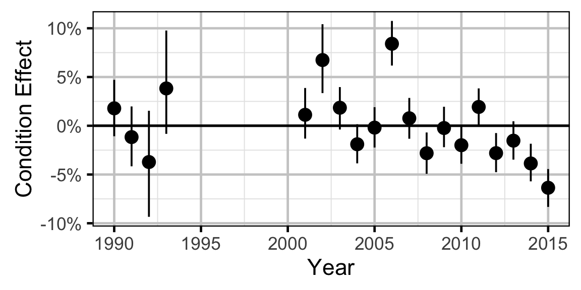
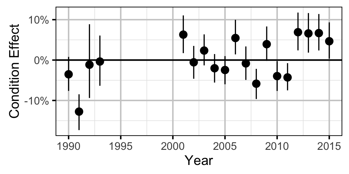
The expected weight of fish of a given length were estimated from the data using a mass-length model (He et al. 2008). Key assumptions of the condition model include:
- The expected weight is allowed to vary with length and date.
- The expected weight is allowed to vary randomly with year.
- The relationship between weight and length is allowed to vary with date.
- The relationship between weight and length is allowed to vary randomly with year.
- The residual variation in weight is log-normally distributed.
Only previously untagged fish were included in models to avoid potential effects of tagging on body condition. Preliminary analyses indicated that the annual variation in weight was not correlated with the annual variation in the relationship between weight and length.
Growth
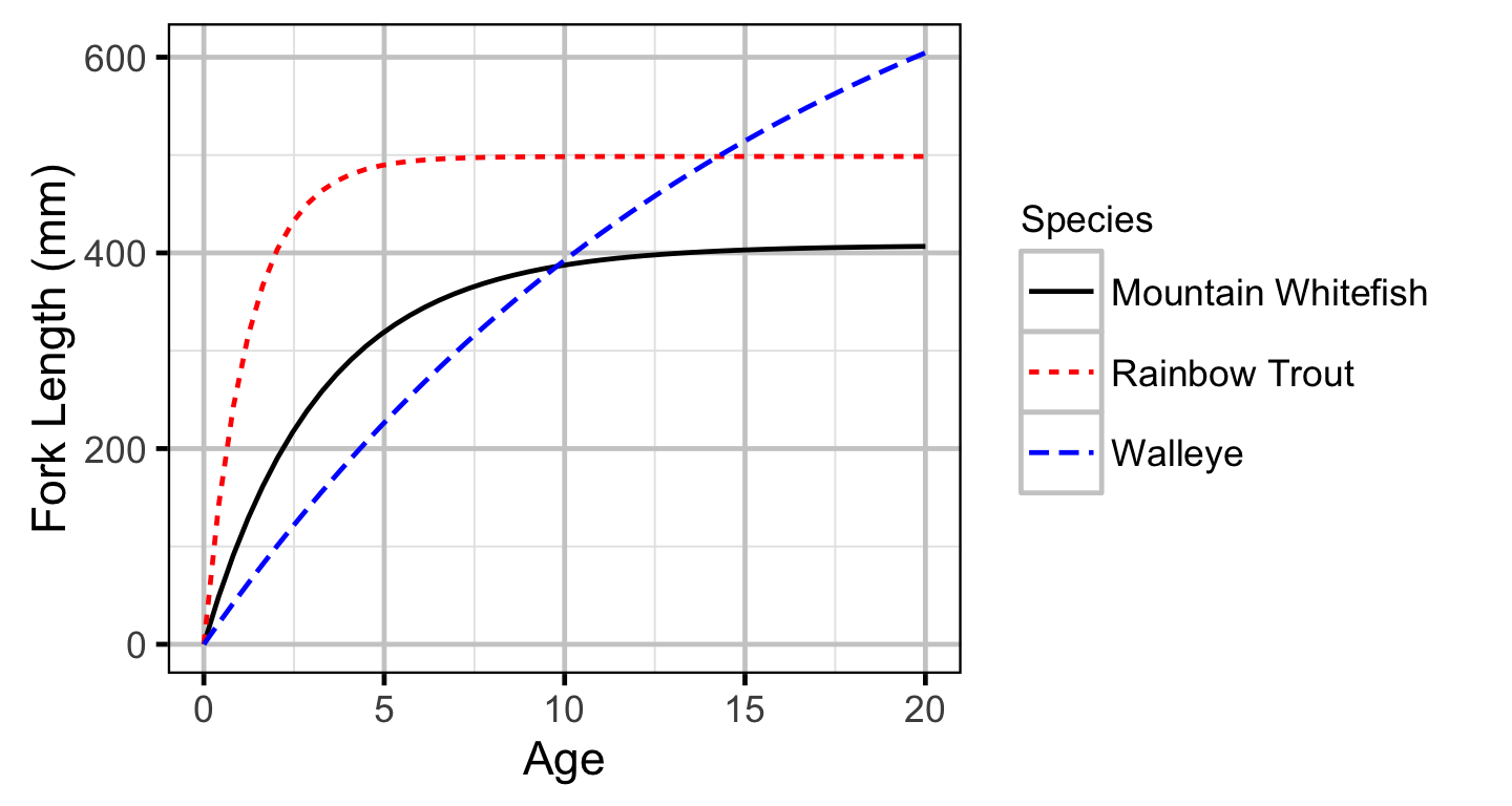
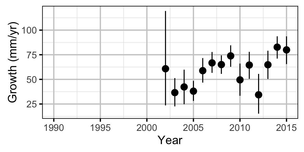
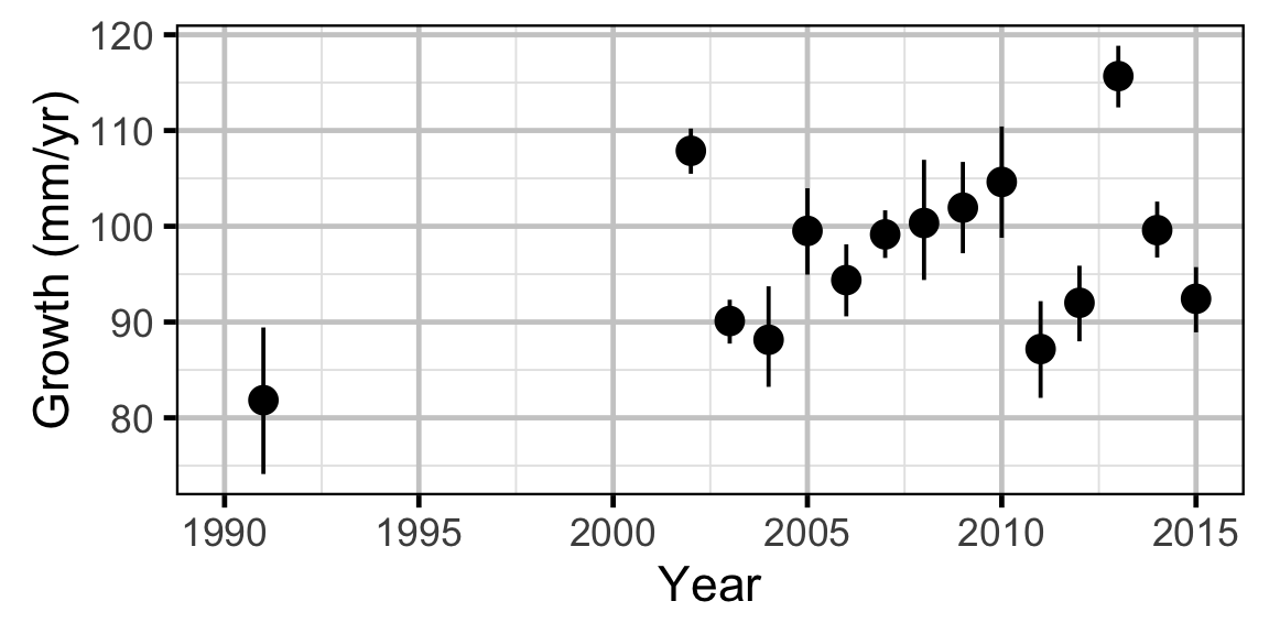
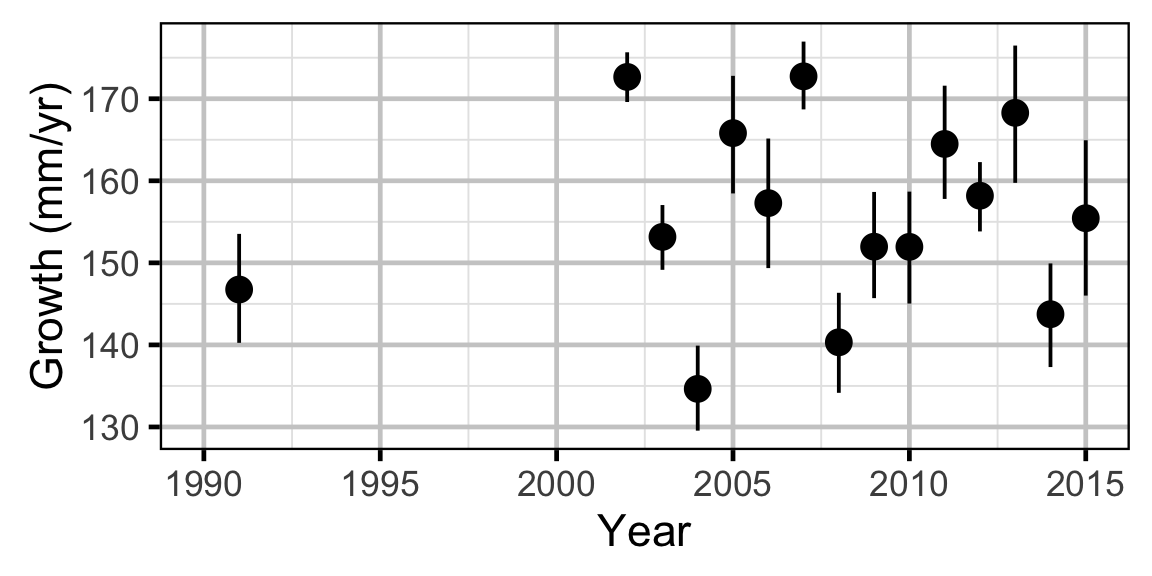
Annual growth of fish were estimated from the inter-annual recaptures using the Fabens method (Fabens 1965) for estimating the von Bertalanffy growth curve (von Bertalanffy 1938). This curve is based on the premise that:
\[ \frac{\text{d}L}{\text{d}t} = k (L_{\infty} - L)\]
where \(L\) is the length of the individual, \(k\) is the growth coefficient and \(L_{\infty}\) is the mean maximum length.
Integrating the above equation gives:
\[ L_t = L_{\infty} (1 - e^{-k(t - t_0)})\]
where \(L_t\) is the length at time \(t\) and \(t_0\) is the time at which the individual would have had no length.
The Fabens form allows
\[ L_r = L_c + (L_{\infty} - L_c) (1 - e^{-kT})\]
where \(L_r\) is the length at recapture, \(L_c\) is the length at capture and \(T\) is the time between capture and recapture.
Key assumptions of the growth model include:
- The mean maximum length \(L_{\infty}\) is constant.
- The growth coefficient \(k\) is allowed to vary randomly with year.
- The residual variation in growth is normally distributed.
Length-At-Age
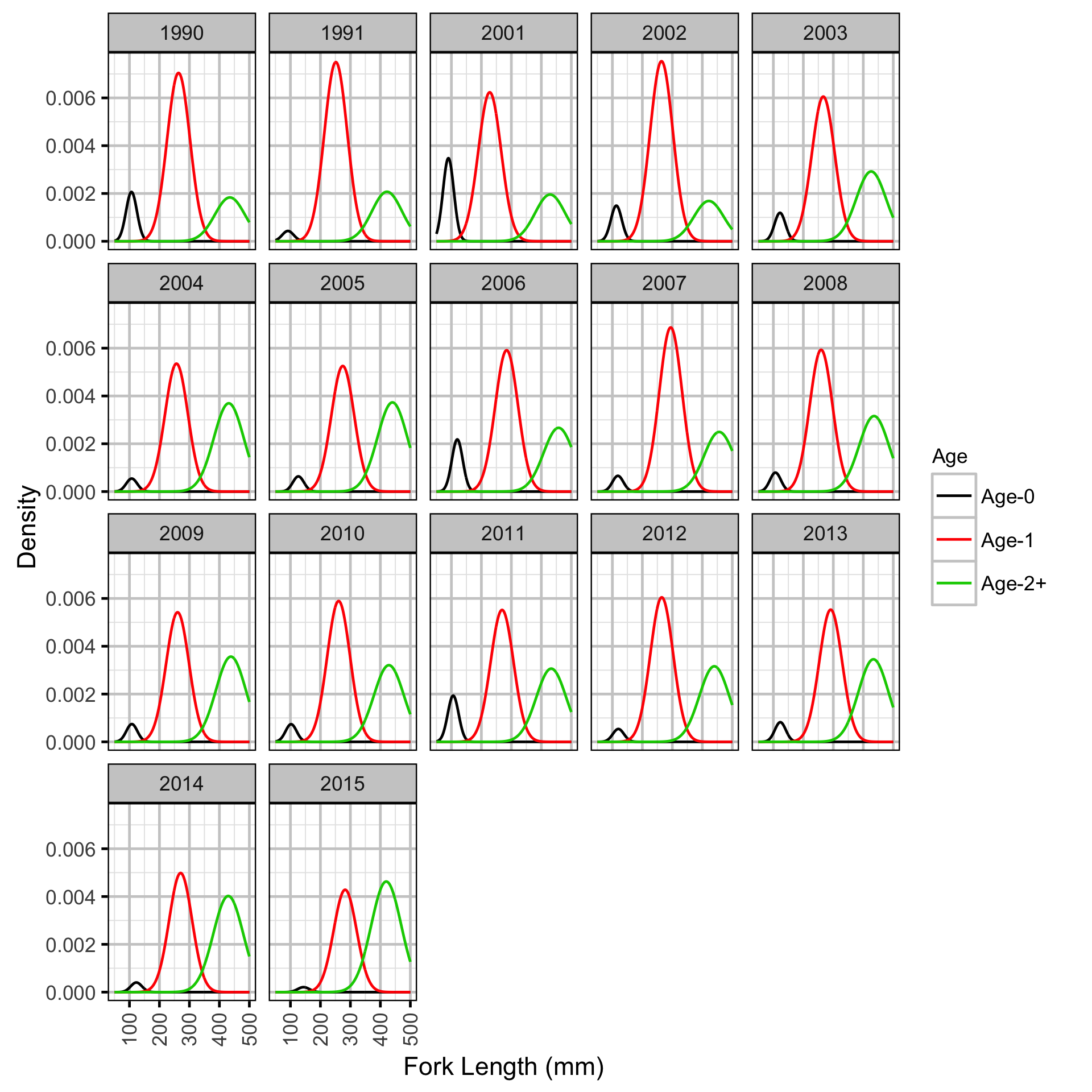
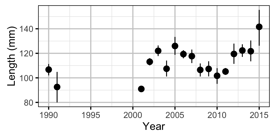
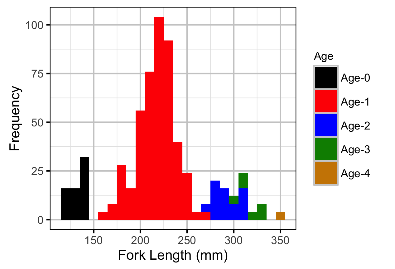
The expected length-at-age of Mountain Whitefish and Rainbow Trout were estimated from annual length-frequency distributions using a finite mixture distribution model (Macdonald and Pitcher 1979). Key assumptions of the length-at-age model include:
- There are three distinguishable age-classes for each species: Age-0, Age-1 and Age-2+.
- The proportion of fish in each age-class is allowed to vary randomly with year.
- The expected growth between age-classes is allowed to vary with age-class.
- The expected growth between age-classes is allowed to vary randomly with age-class within year.
- The expected length increases with age-class.
- The expected length is allowed to vary with year within age-class.
- The expected length is allowed to vary as a second-order polynomial with date.
- The relationship between length and date is allowed to vary randomly with age-class.
- The residual variation in length is normally distributed.
- The standard deviation of this normal distribution is allowed to vary randomly with age-class.
The model was used to estimate the cut-offs between age-classes by year. For the purposes of estimating other population parameters by age-class, Age-0 individuals were classified as fry, Age-1 individuals were classified as subadult, and Age-2+ individuals were classified as adult. Walleye could not be separated by life stage due to a lack of discrete modes in the length-frequency distributions for this species. Consequently, all captured Walleye were considered to be adults.
The results include plots of the age-class density for each year by length as predicted by the length-at-age model. Density is a measure of relative frequency for continuous values.
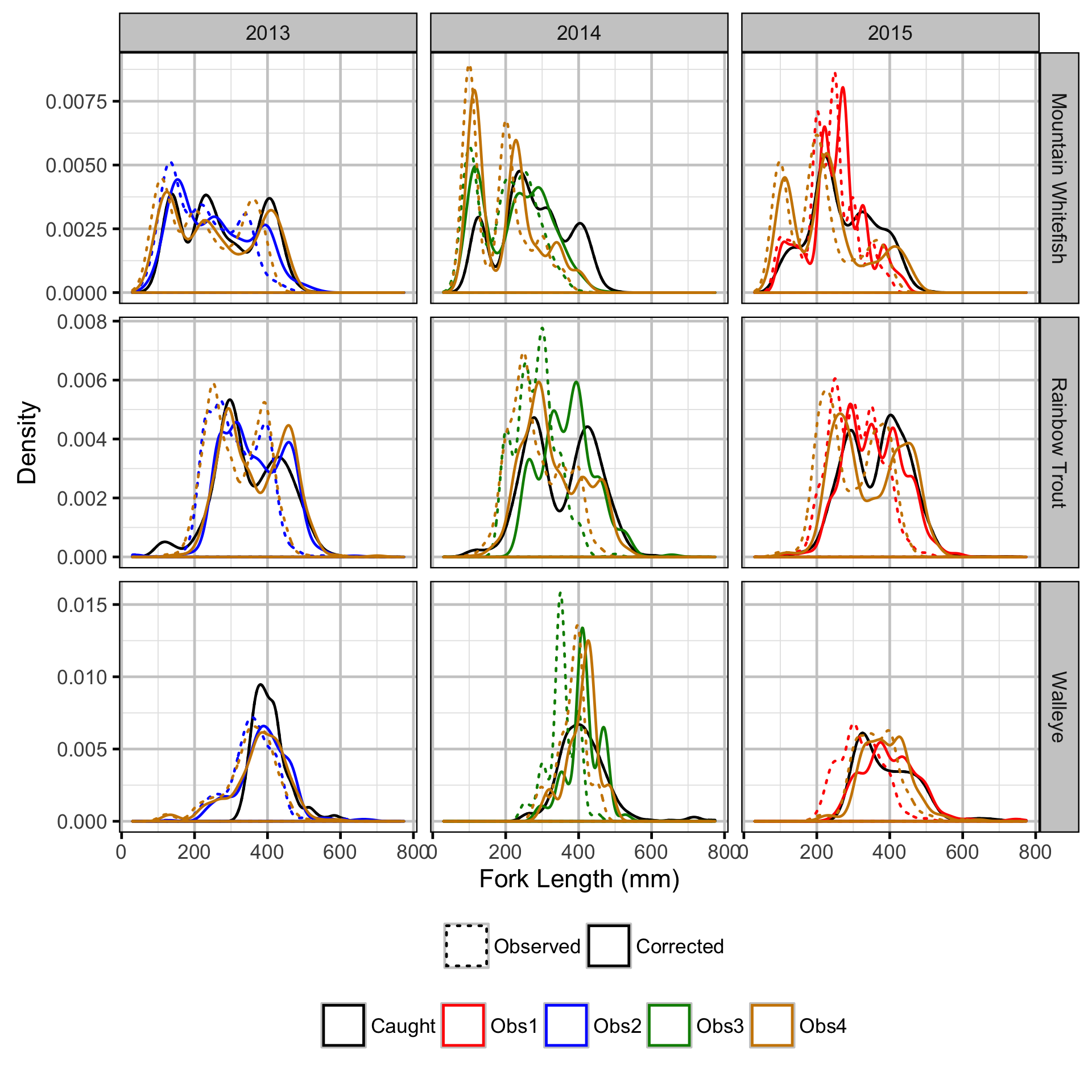
Observer Length Correction
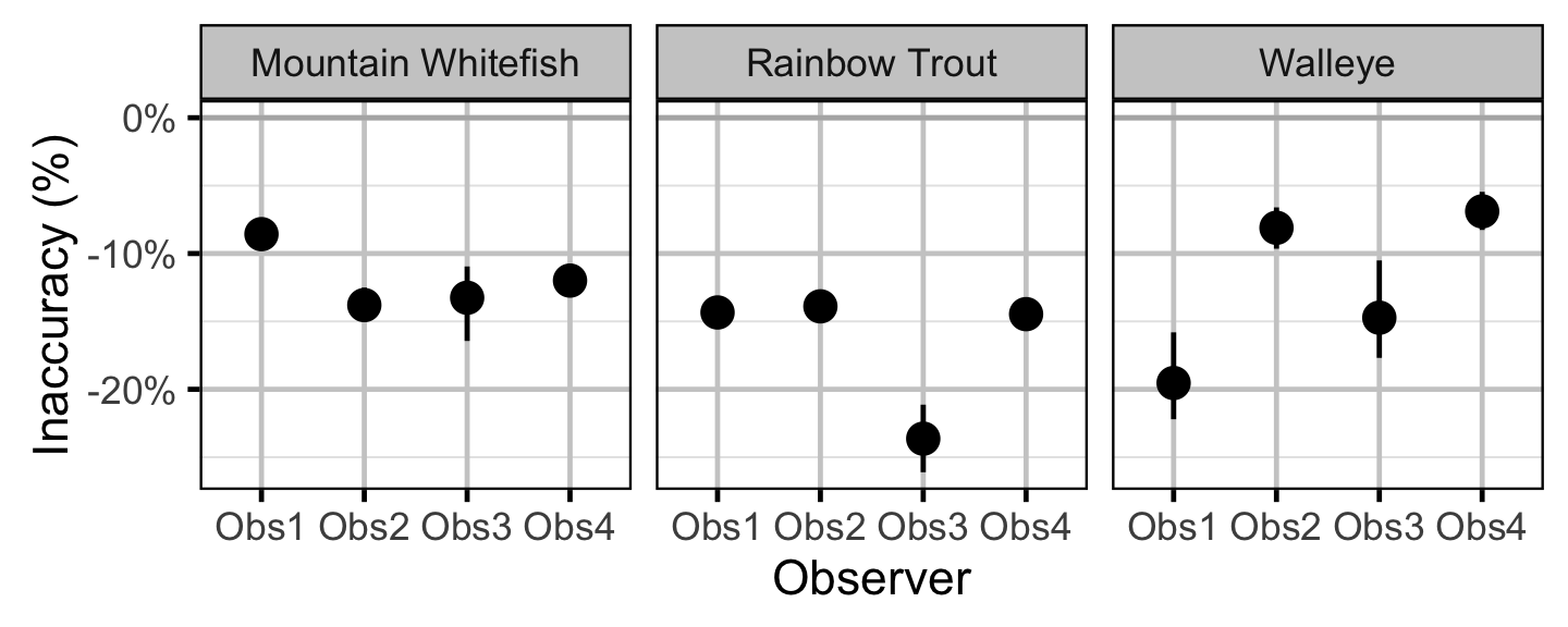
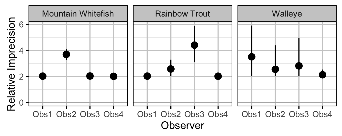
The bias (accuracy) and error (precision) in observer’s fish length estimates were quantified using a model with a categorical distribution which compared the proportions of fish in different length-classes for each observer to the equivalent proportions for the measured fish. Key assumptions of the observer length correction model include:
- The proportion of fish in each length-class is allowed to vary with year.
- The expected length bias is allowed to vary with observer.
- The expected length error is allowed to vary with observer.
- The expected length bias and error for a given observer does not vary by year.
- The residual variation in length is normally distributed.
The observed fish lengths were corrected for the estimated length biases before being classified as fry, subadult and adult based on the length-at-age cutoffs.
Survival
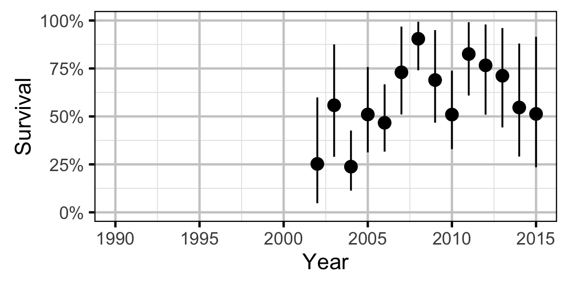
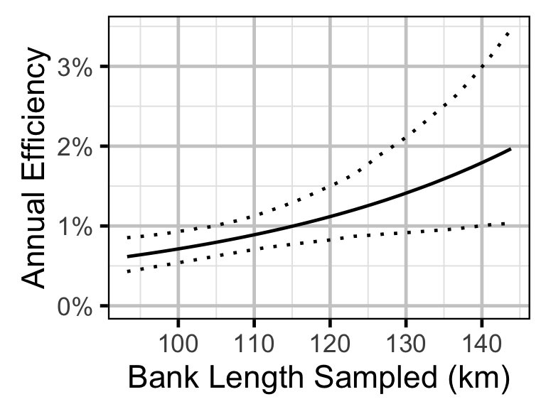
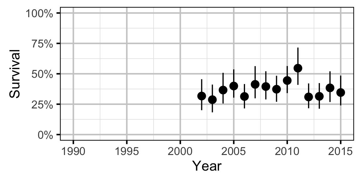
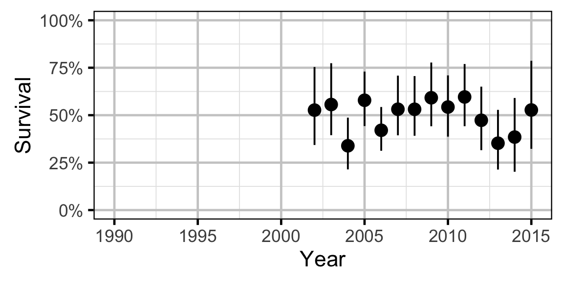
The annual adult survival rate was estimated by fitting a Cormack-Jolly-Seber model (Kery and Schaub 2011, 220–31) to inter-annual recaptures of adults.
Key assumptions of the survival model include:
- Survival varies randomly with year.
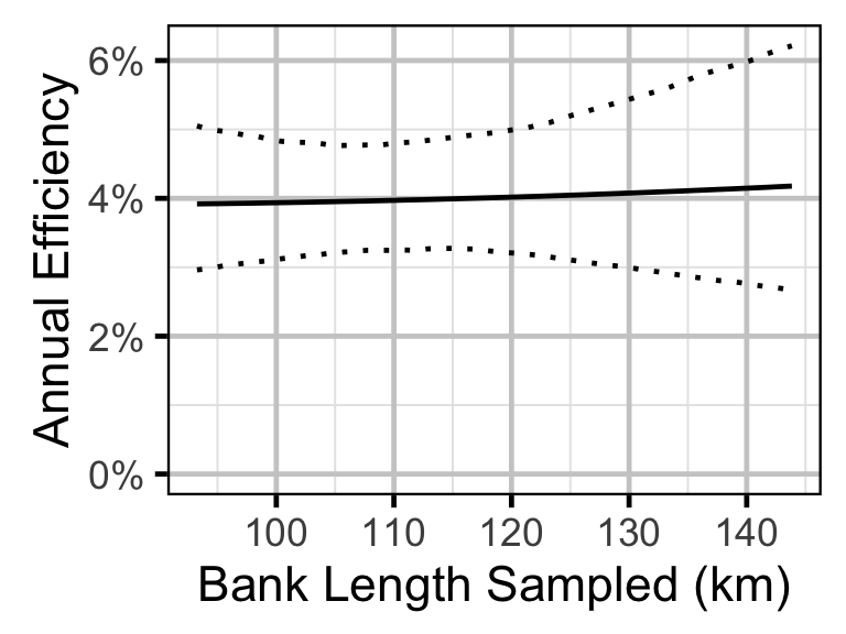
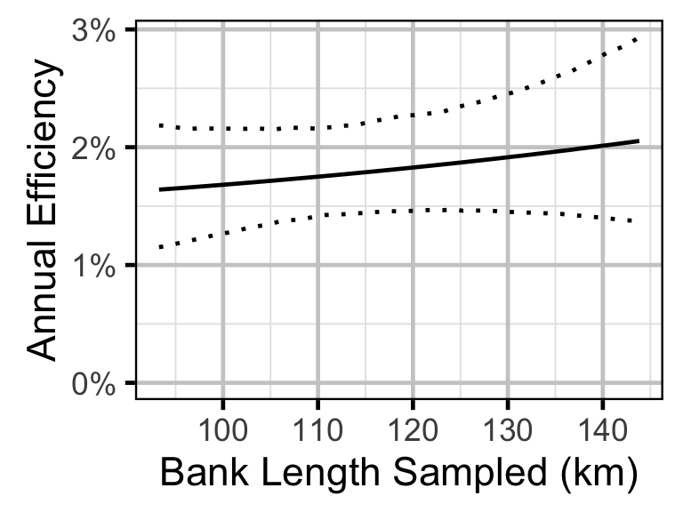
- The encounter probability for adults is allowed to vary with the total bank length sampled.
Site Fidelity
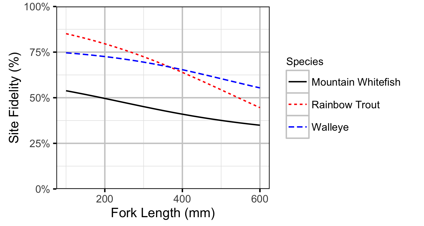
The extent to which sites are closed, i.e., fish remain at the same site between sessions, was evaluated with a logistic ANCOVA (Kery 2010). The model estimates the probability that intra-annual recaptures were caught at the same site versus a different one. Key assumptions of the site fidelity model include:
- The expected site fidelity is allowed to vary with fish length.
- Observed site fidelity is Bernoulli distributed.
Length as a second-order polynomial was not found to be a significant predictor for site fidelity.
Capture Efficiency
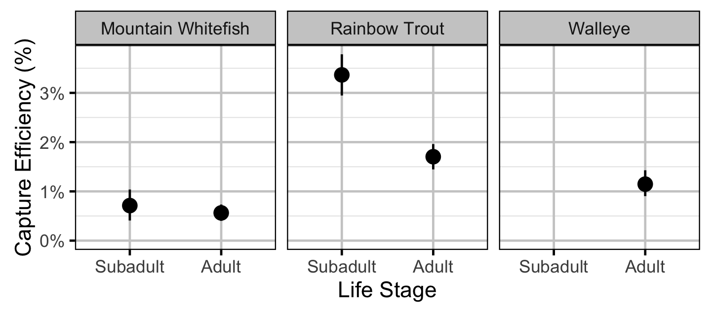
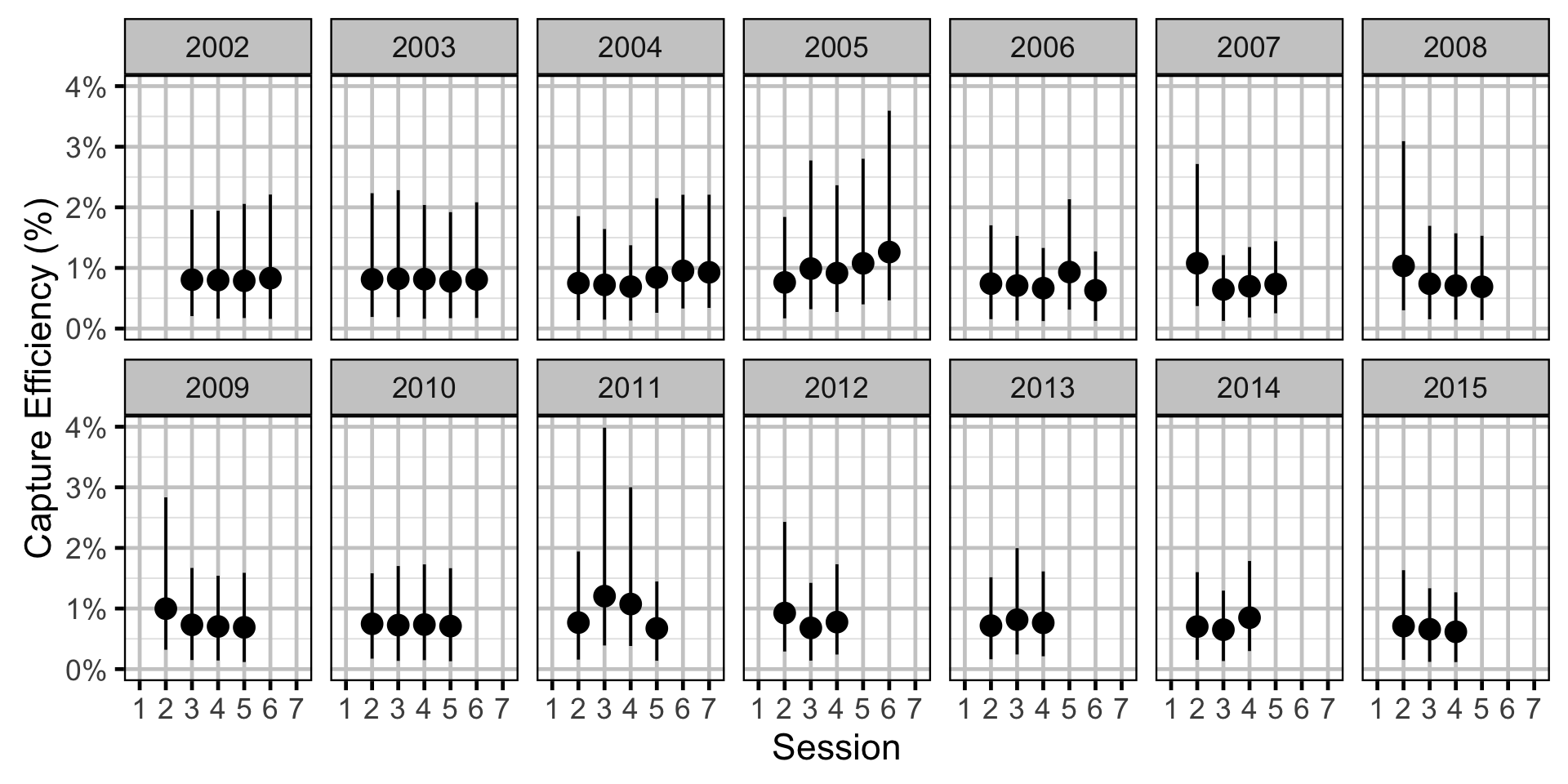
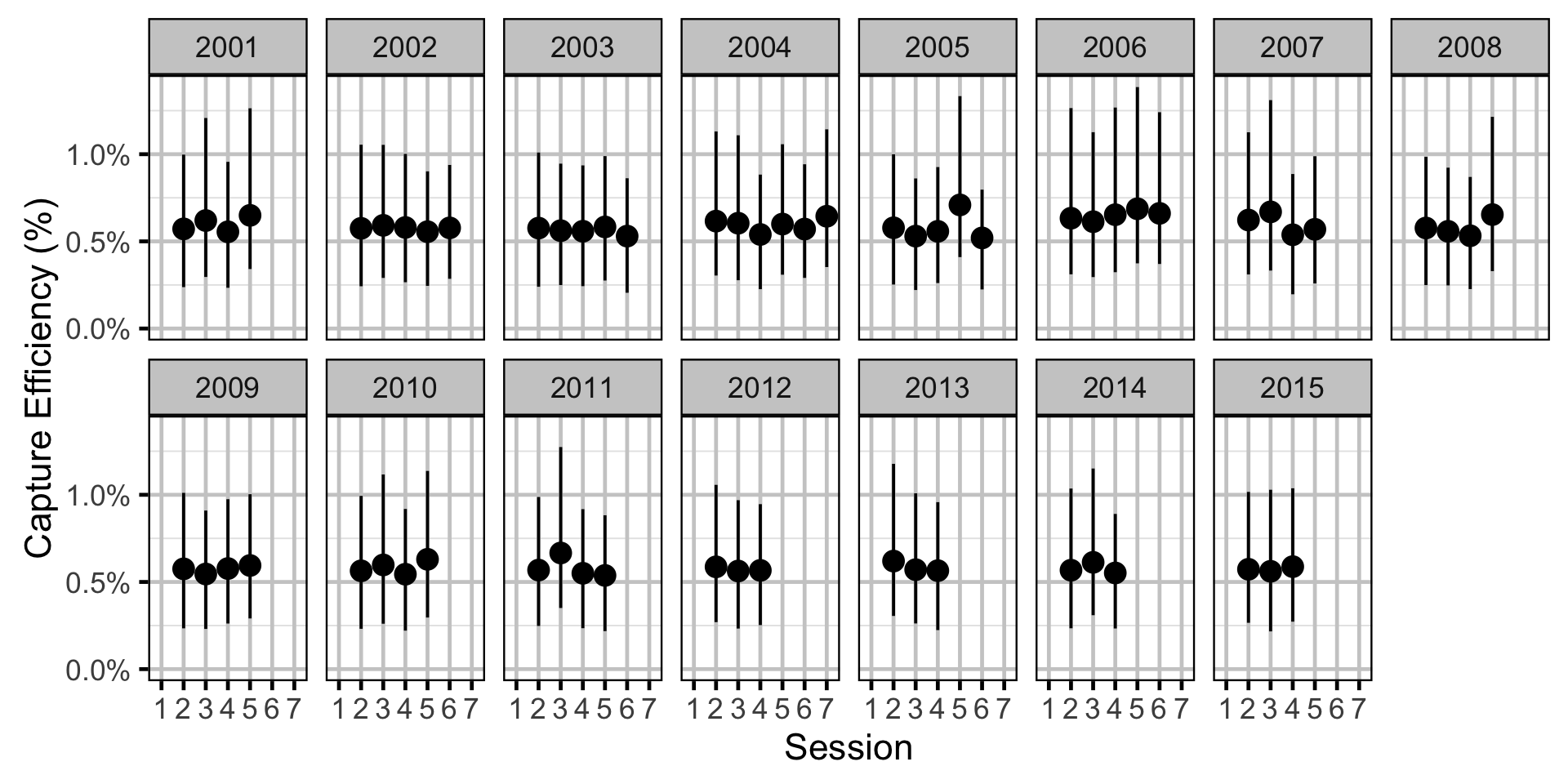
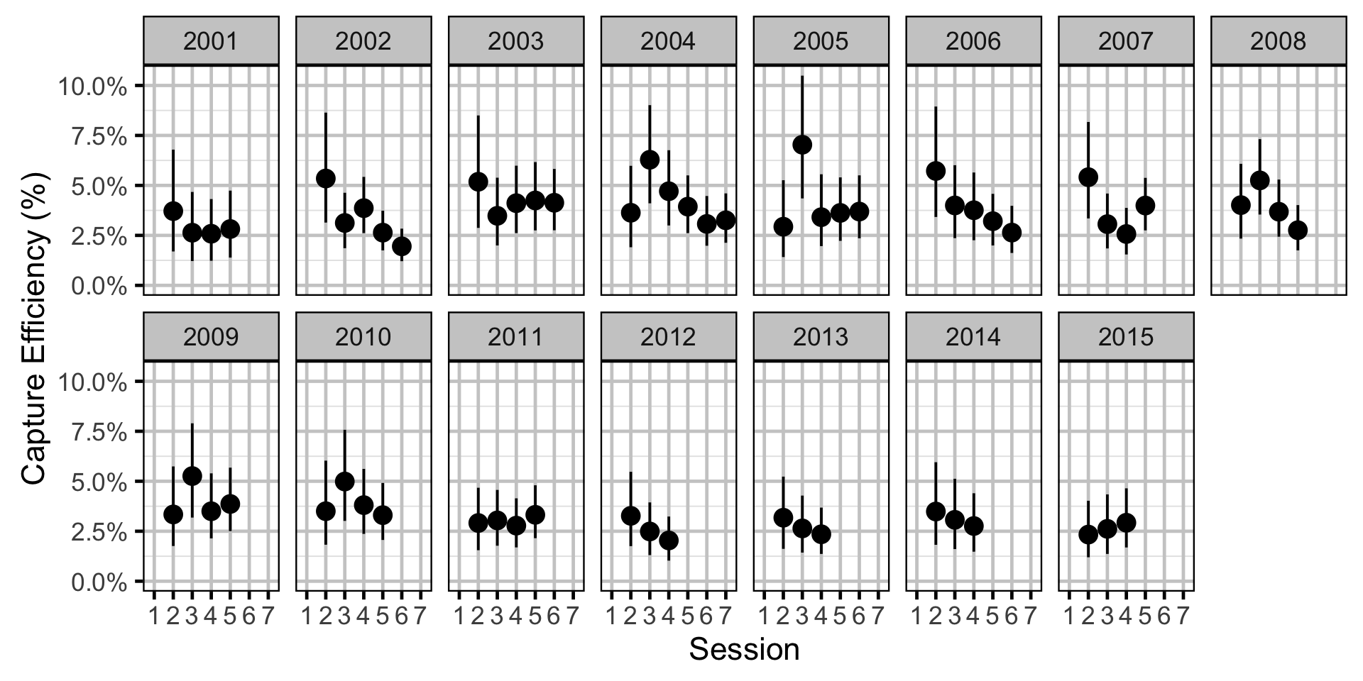
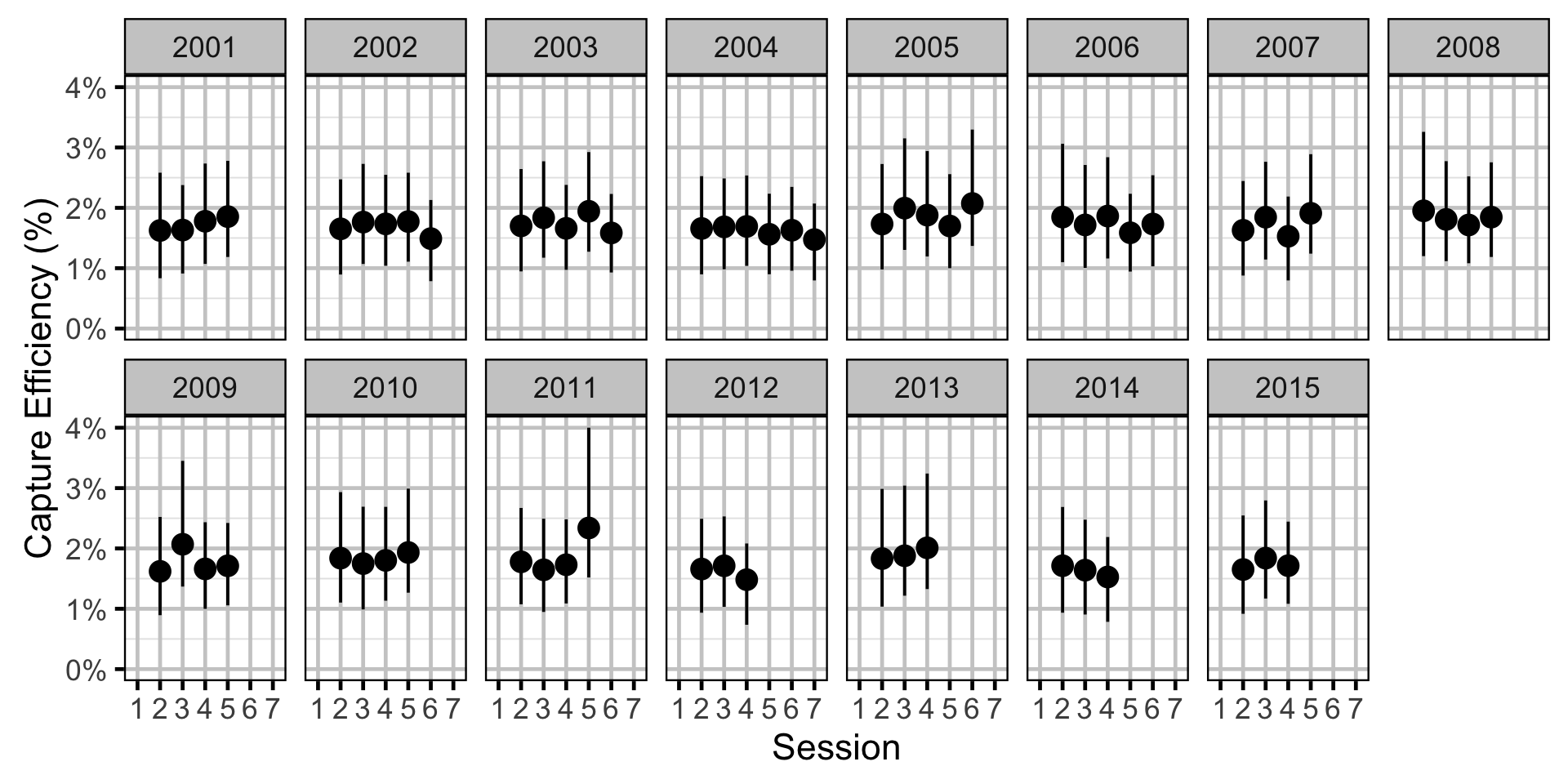
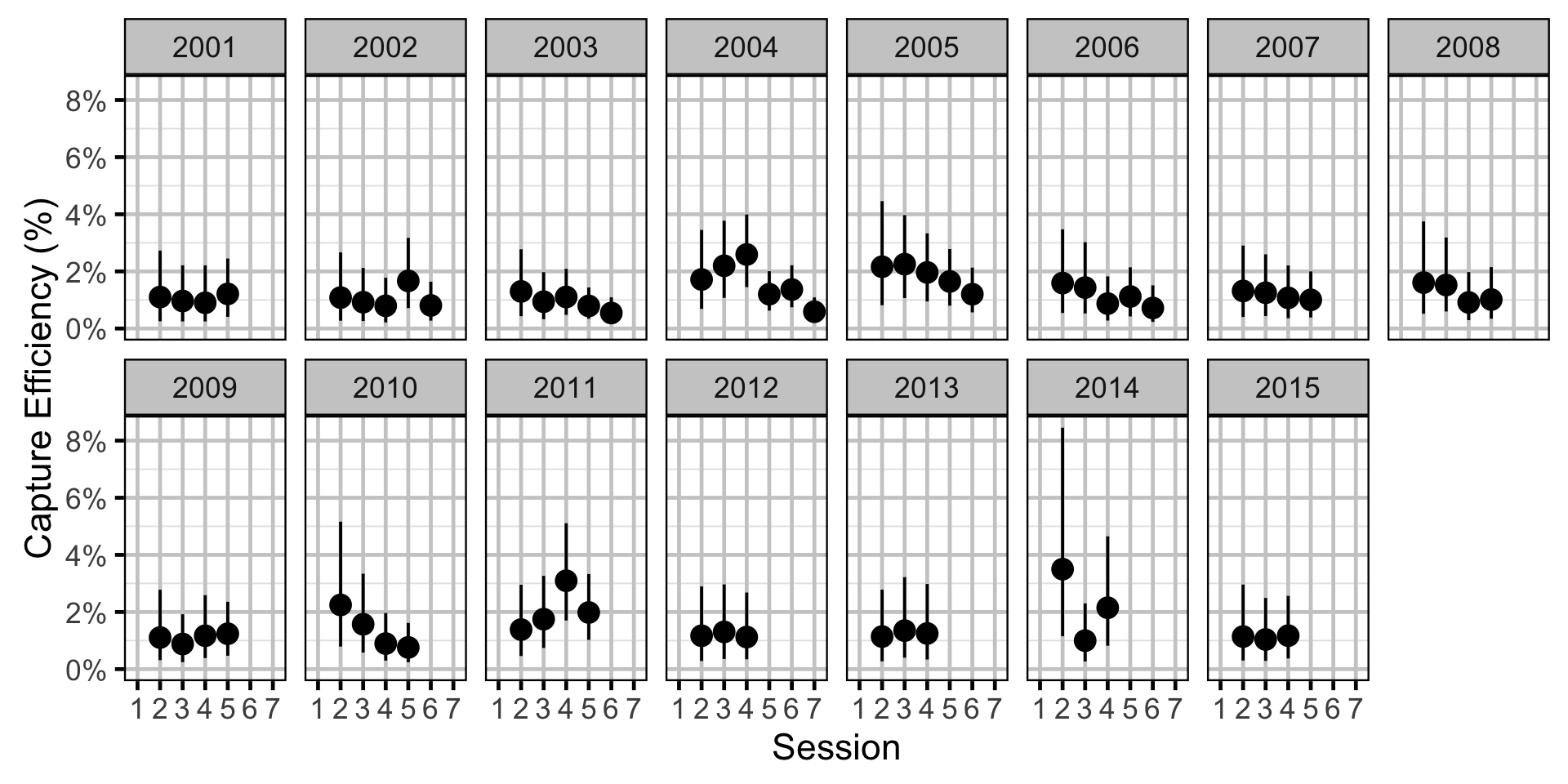
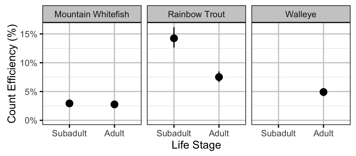
The probability of capture was estimated using a recapture-based binomial model (Kery and Schaub 2011, 134–36, 384–88).
Key assumptions of the capture efficiency model include:
- The capture probability varies randomly by session within year.
- The probability of a marked fish remaining at a site is the estimated site fidelity.
- The number of recaptures is described by a binomial distribution.
Abundance
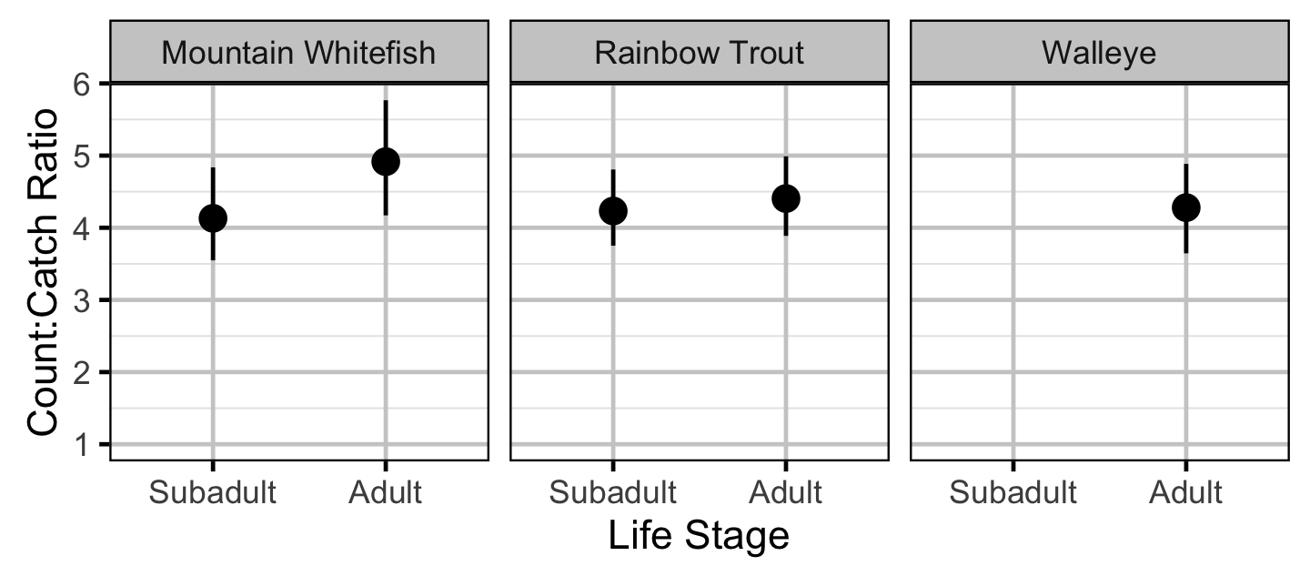
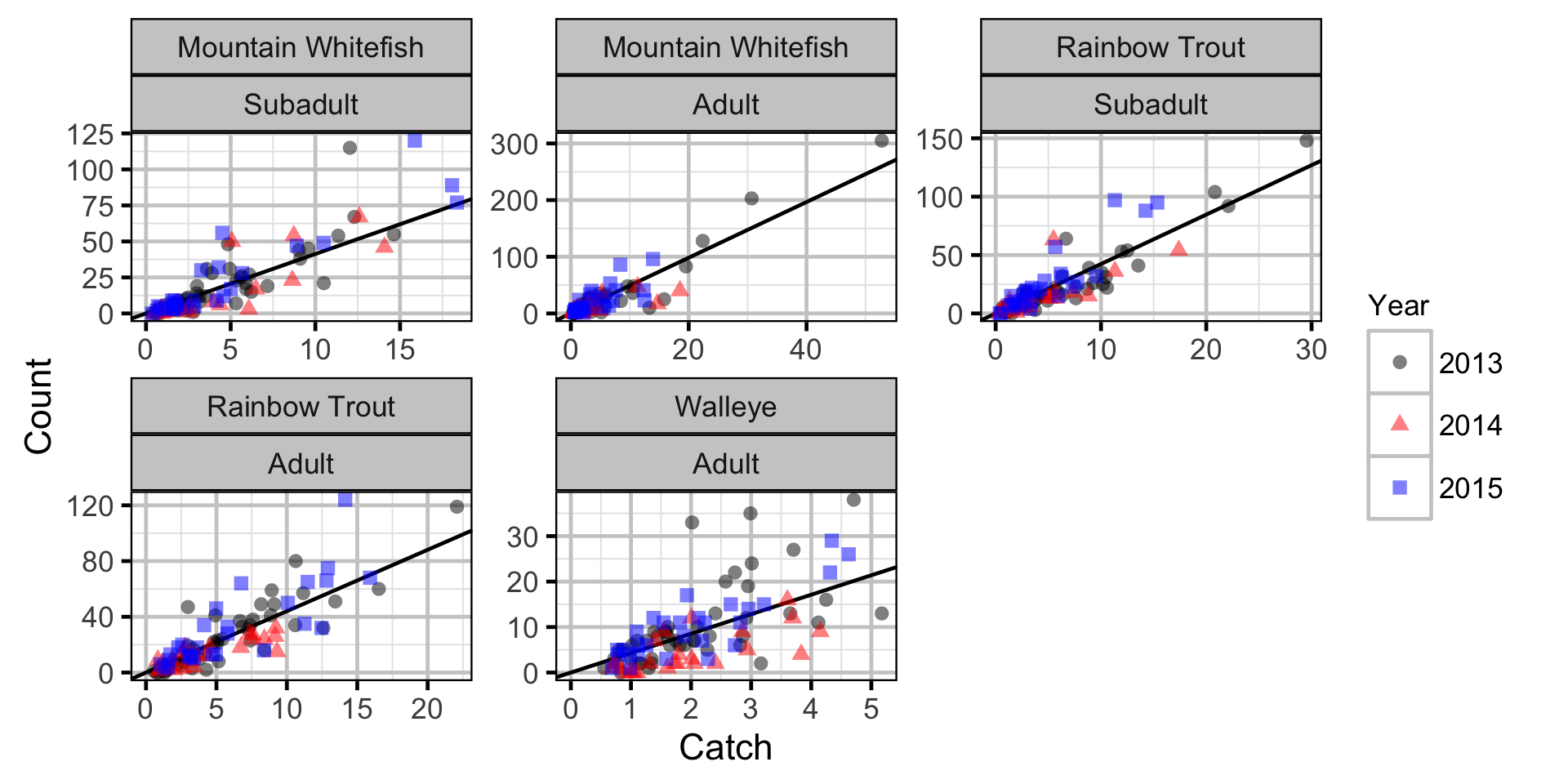
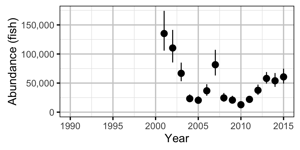
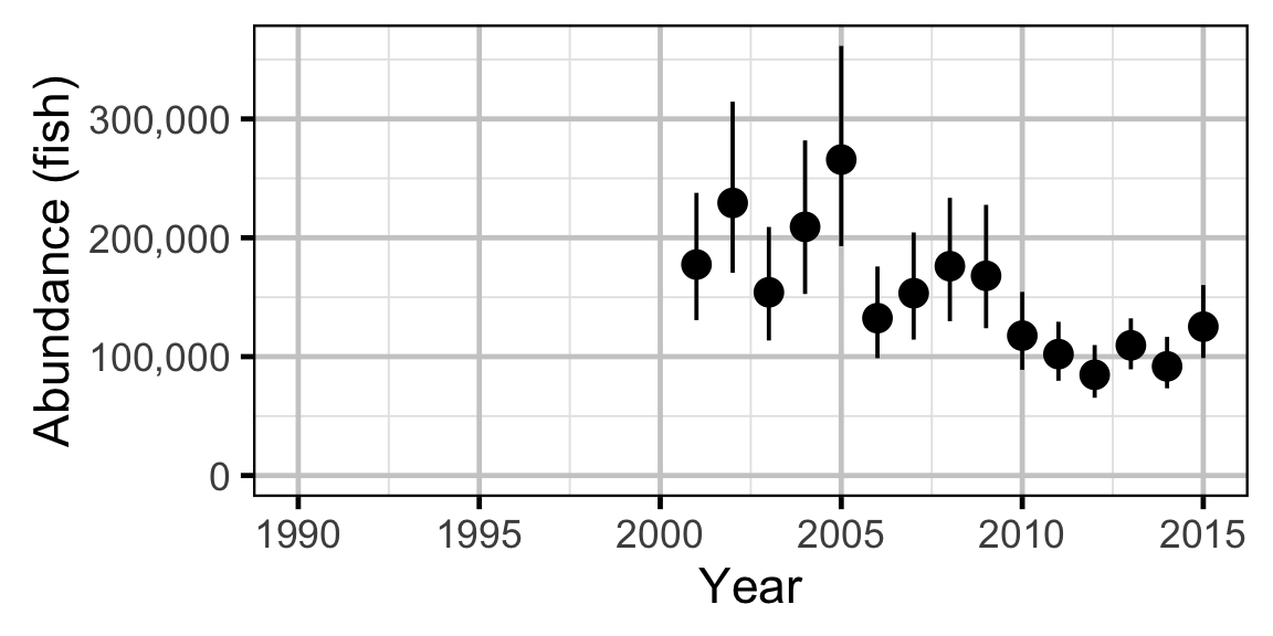
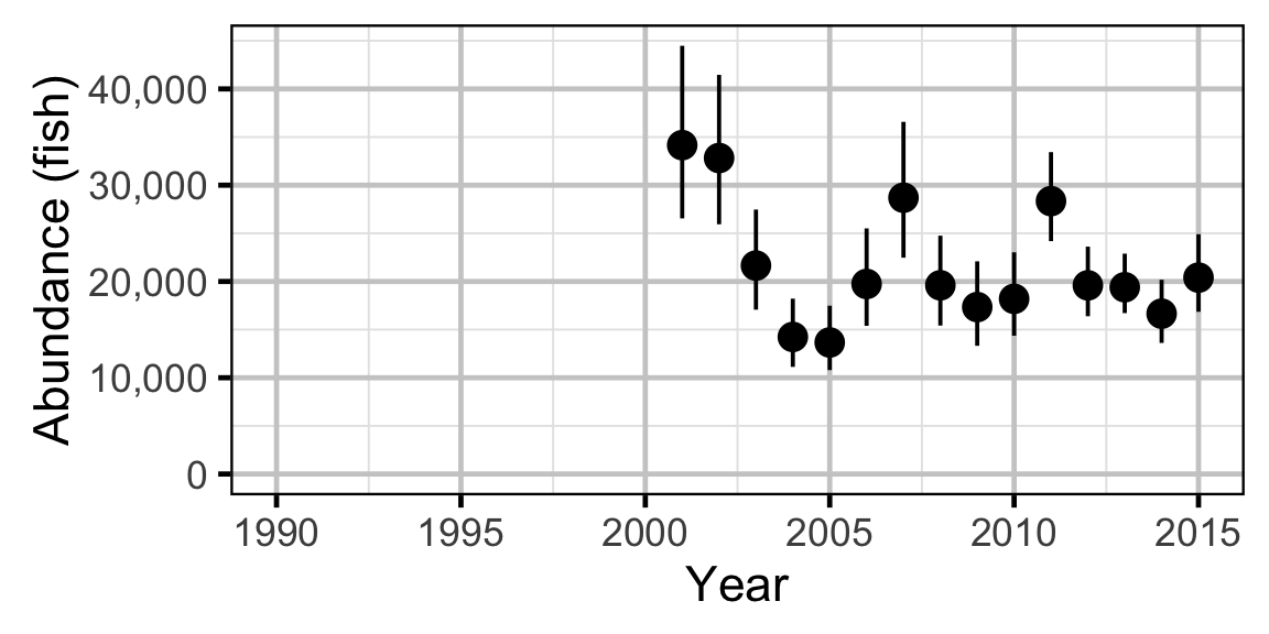
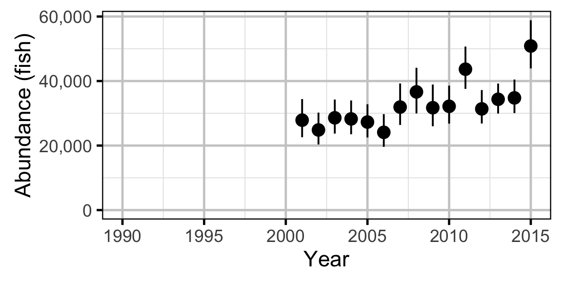
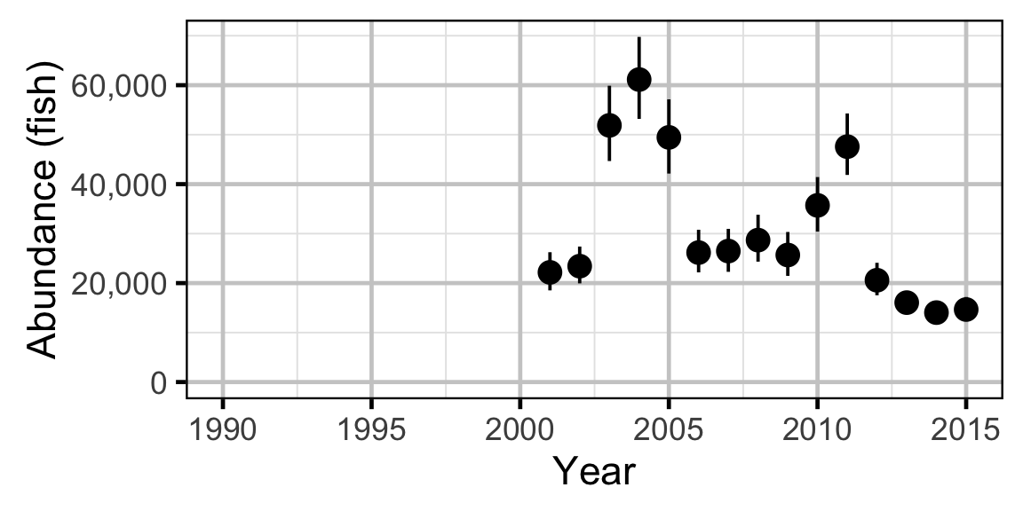
The abundance was estimated from the catch and bias-corrected observer count data using an overdispersed Poisson model (Kery and Schaub 2011, 55–56). The model assumed that the capture efficiency was the mean estimate from the capture efficiency model and that the number of observed fish was a multiple of the number of captured fish. The annual abundance estimates represent the total number of fish in the study area.
Key assumptions of the abundance model include:
- The capture efficiency is the mean estimate from the capture efficiency model.
- The observer efficiency varies from the capture efficiency.
- The lineal fish density varies randomly with site, year and site within year.
- The catches and counts are described by a Poisson-gamma distribution.
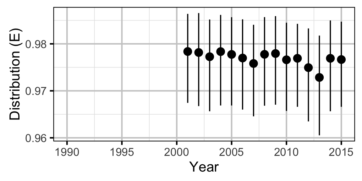
The annual distribution of each species was calculated using the Shannon index of evenness (\(E\)) where \(S\) was the number of sites and \(p_i\) the proportion of the population belonging to the \(i\)th site.
\[ E = \frac{-\sum p_i \log(p_i)}{ln(S)}\]
Long-Term Trends
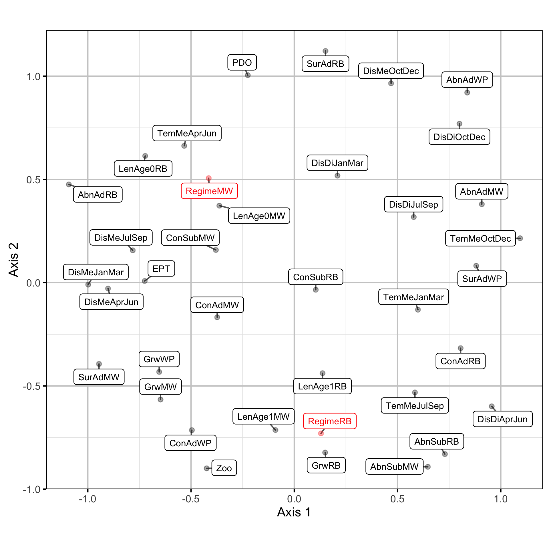
Trends common to the fish index and environmental annual time series were identified using dynamic factor analysis (DFA) (Zuur, Tuck, and Bailey 2003) – a dimension-reduction technique designed for time-series data.
The fish index time series were the condition (Con), growth (Grw) length-at-age (Len), survival (Sur) and Abundance (Abn) by species (MW = Mountain Whitefish, RB = Rainbow Trout, WP = Walleye) and life stage (Sub = Subadult, Ad = Adult) or age (Age0, Age1).
The environmental time series were the mean (DisMe) and average hourly absolute difference (DisDi) in discharge at Birchbank, the average water temperature (TemMe) at Norns Creek by quarterly period, the Pacific Decadal Oscillation Index (PDO), the Ephemeroptera, Plecoptera, Trichoptera and Dipterans in the Lower Columbia River (EPT), the biomass of zooplankton in Arrow Lakes Reservoir (ZOO) and the annual proportional egg loss through dewatering (Regime) by species (MW = Mountain Whitefish, RB = Rainbow Trout).
The average hourly absolute discharge difference was calculated by differencing the mean hourly discharge time series and taking the average of the absolute differences. Mathematically this is equivalent to: \[ \frac{\sum |x_{1}-x_{2}| + |x_{2}-x_{3}| + ... + |x_{n-1}-x_{n}|}{n-1} \] where \(x_{1}\) is the discharge at the start of the time series and \(x_{2}\) is the discharge an hour later.
The October to December times series were lead by one year to account for the fact that they occurred after sampling and are expected to only influence the fish time series in the following year. Similarly, the Mountain Whitefish egg loss time series were also lead by one year to account for the fact that they flow changes mostly occur the following year. If \(\geq\) 10% of the discharge or temperature data were missing for a three-month period the value was not included in the time series.
All time series were standardized prior to fitting the DFA model. Key assumptions of the model include:
- The time series are described by six underlying trends.
- The random walk processes in the trends are normally distributed.
- The residual variation in the standardised variables is normally distributed.
Due to the rotation problem the underlying trends were indeterminate (Abmann, Boysen-Hogrefe, and Pape 2014). The similarities were represented visually by using non-metric multidimensional scaling (NMDS) to cluster the time series based on the absolute values of the dynamic factor analysis trend weightings.
Short-Term Correlations
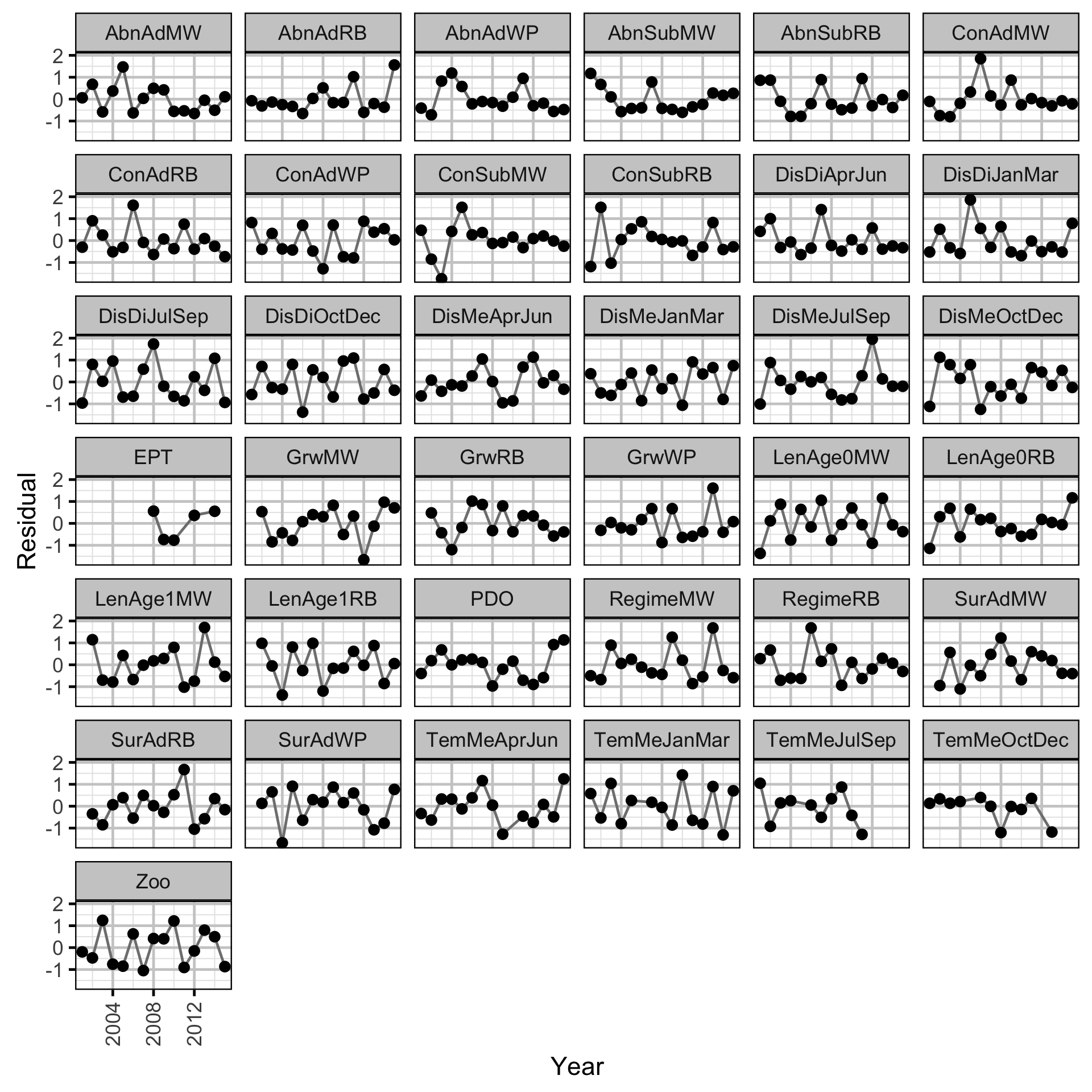
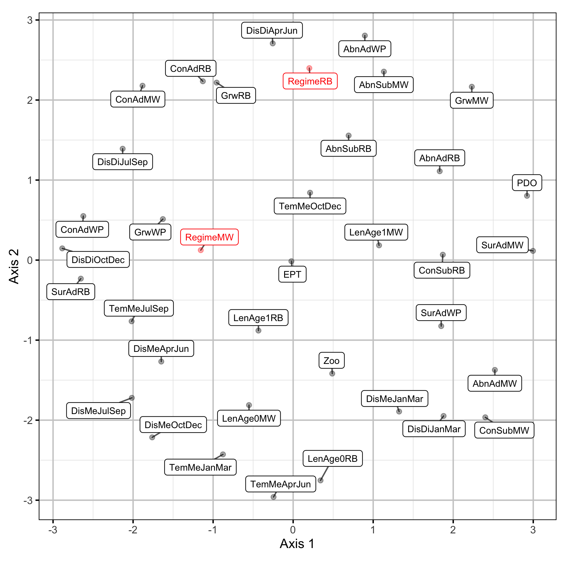
To assess the short-term congruence between the yearly fish metrics and the environmental variables, the pair-wise distances between the residuals from the DFA model were calculated as \(1 - |\rho(x, y)|\) where \(\rho\) is the Pearson correlation and \(x\) and \(y\) are the two time series being compared.
The short-term similarities were represented visually by using NMDS to cluster the time series based on the pair-wise distances.
Scale Age
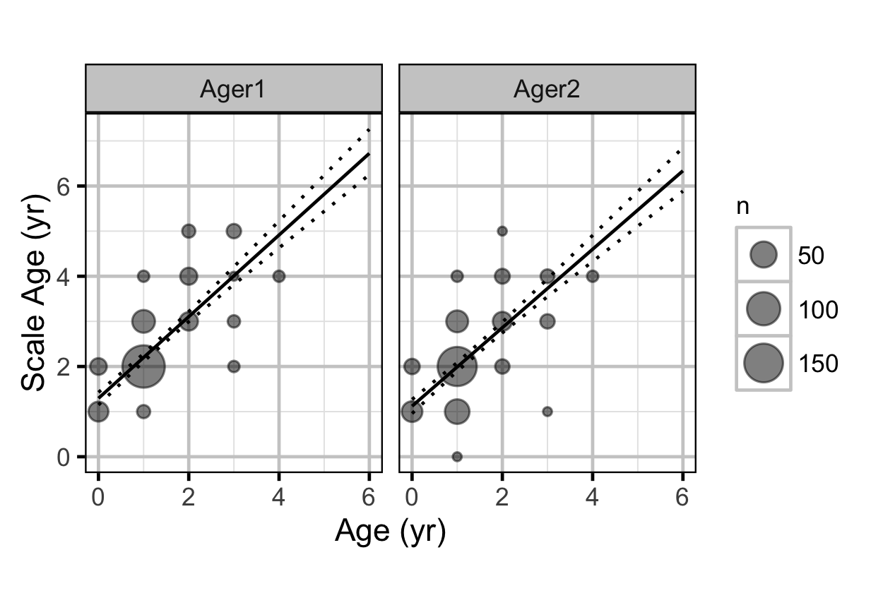
The age of Mountain Whitefish was estimated from scales by two independent agers. The scale aging process was repeated twice per ager, leading to two observations per ager per fish encounter (Hurlbert 1984). Individuals that could be aged at initial capture based on their length using the length-at-age model with a certainty \(\geq 0.95\) were assigned a known hatch year. Otherwise the hatch year was estimated by the model from the scale ages. The scale ages were analysed using a state-space linear mixed model that assigned an age to each fish based on the year of capture and its hatch year.
Key assumptions of the scale age model include:
- The actual age is the year of capture minus the hatch year
- The scale age varies by ager.
- The scale age varies randomly with fish encounter and ager within fish encounter.
- The scale age varies linearly with age.
- The effect of age on scale age varies by ager.
- The random effects are normally distributed.
- The residual variation in the scale ages (replicate within ager within encounter) is described by a zero-truncated normal distribution.
Age-Ratios
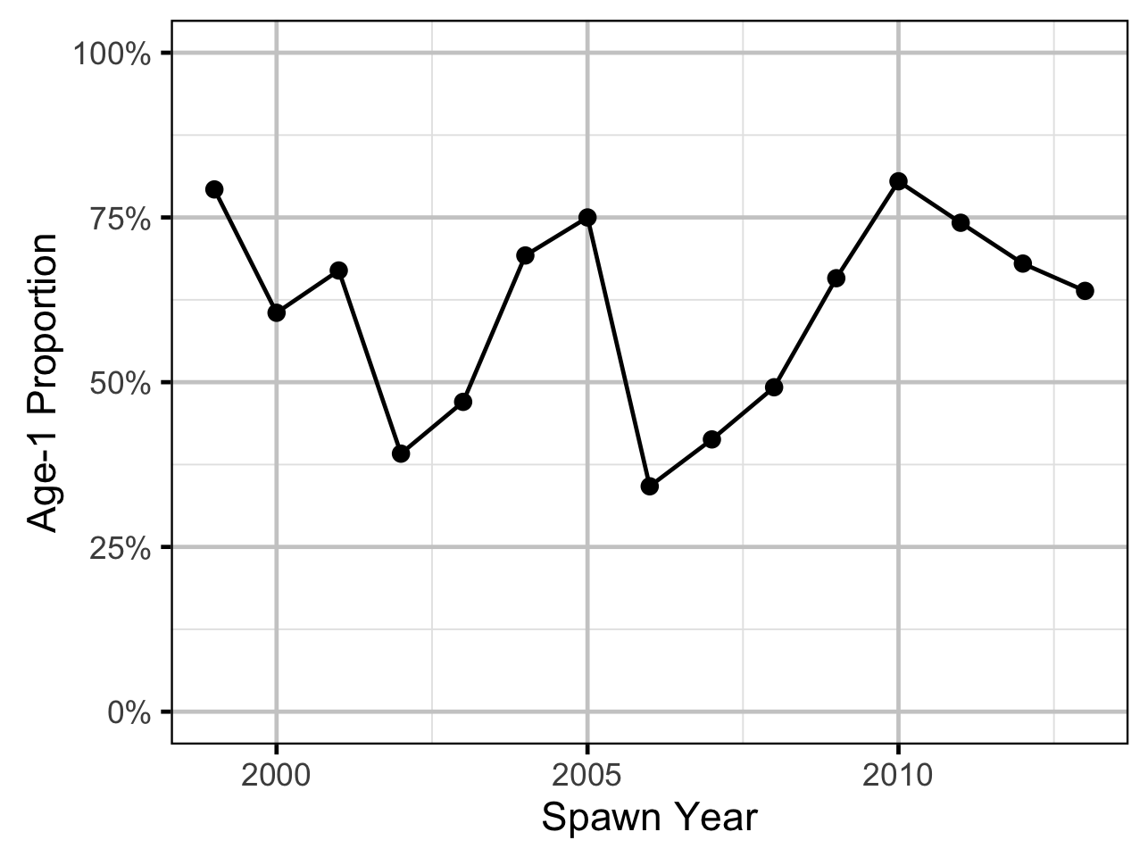
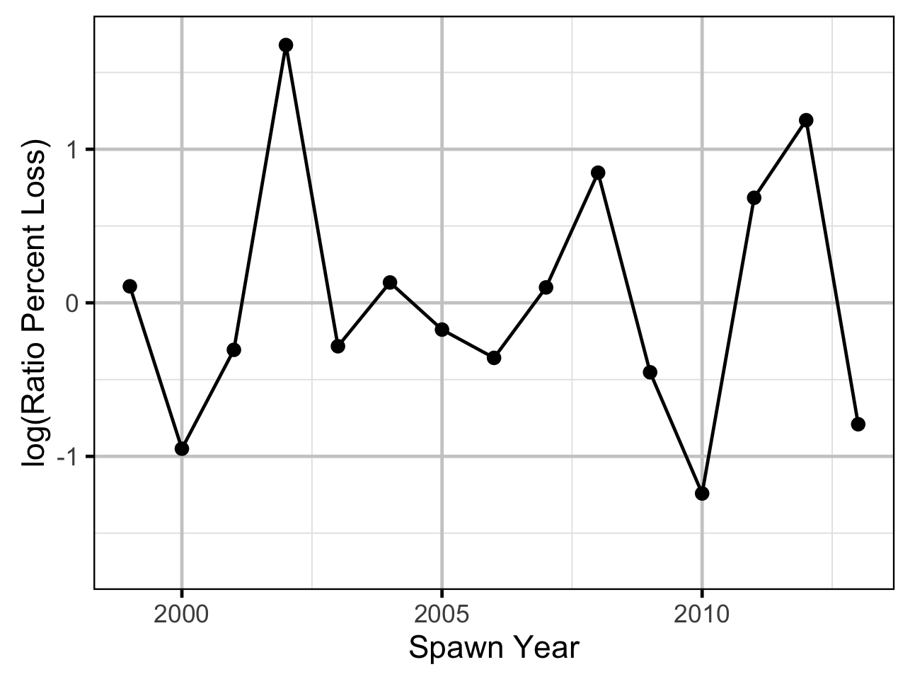
The proportion of Age-1 Mountain Whitefish \(r^1_t\) from a given spawn year \(t\) is calculated from the number of Age-1 and Age-2 fish \(N^1_t\) and \(N^2_t\) respectively, which were lead or lagged so that all values were with respect to the spawn year:
\[r^1_t = \frac{N^1_{t+2}}{N^1_{t+2} + N^2_{t+2}}\]
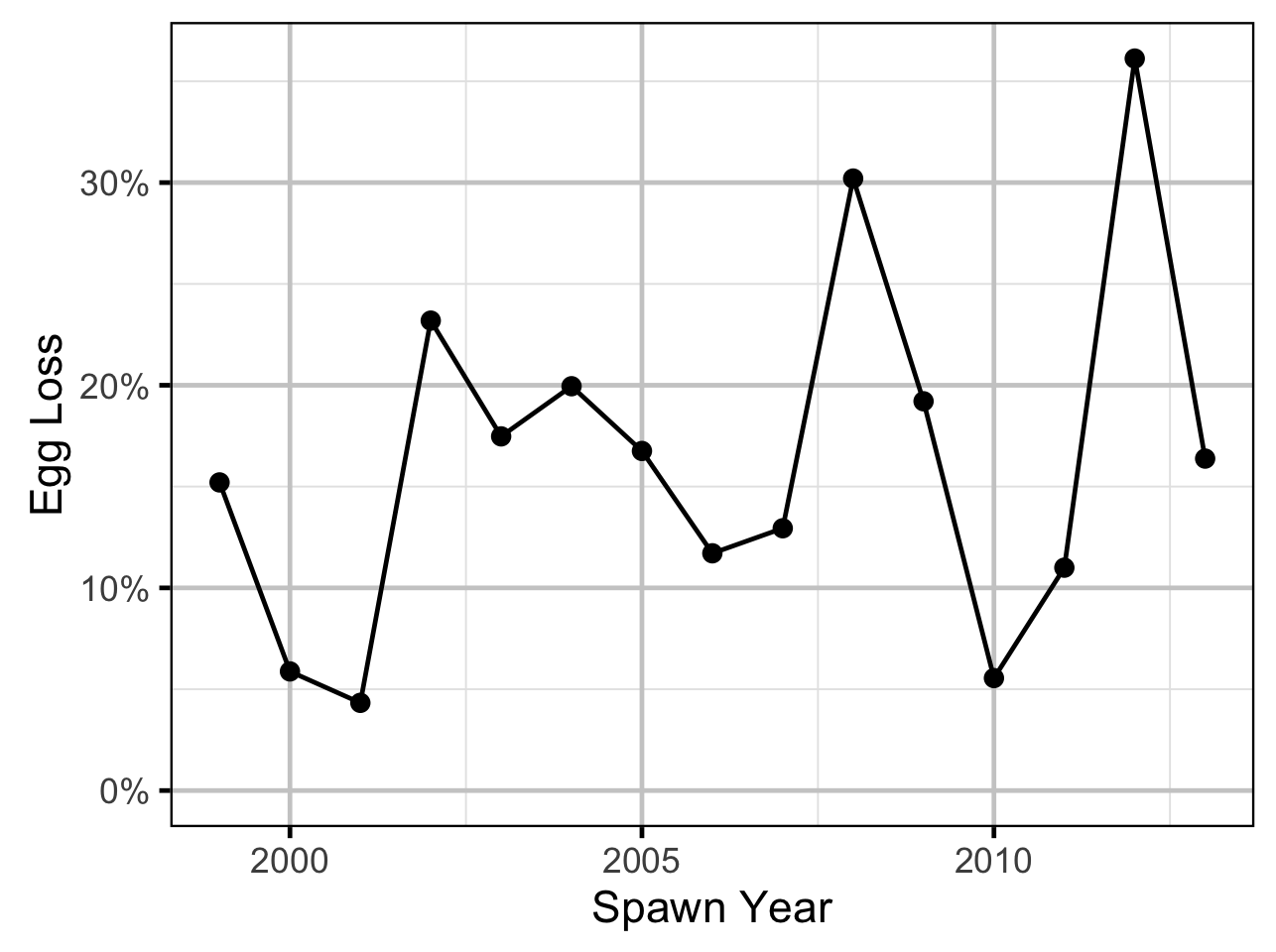
As the number of Age-2 fish might be expected to be influenced by the percentage egg loss \(Q_t\) three years prior, the predictor variable \(\Pi_t\) used is:
\[\Pi_t = \textrm{log}(Q_t/Q_{t-1})\]
The ratio was logged to ensure it was symmetrical about zero (Tornqvist, Vartia, and Vartia 1985). The ages from the scale age model were corrected by subtracting one.
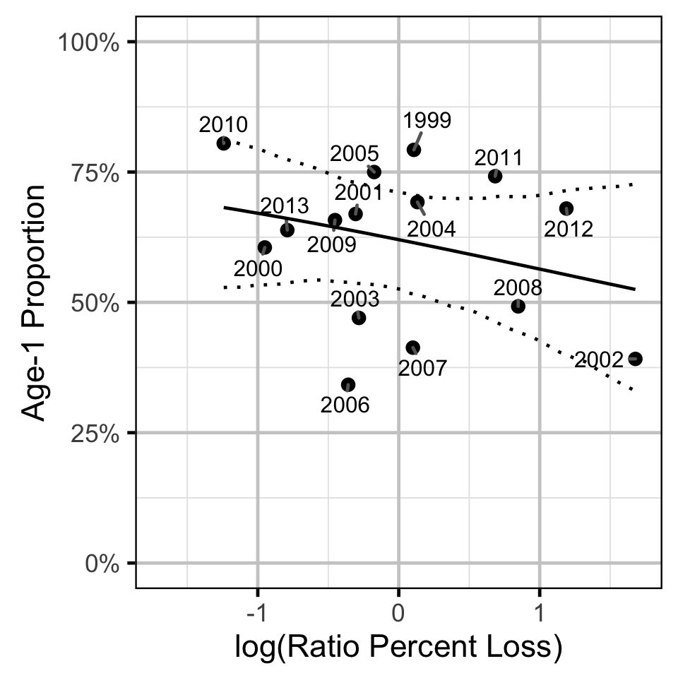
The relationship between \(r^1_t\) and \(\Pi_t\) was estimated using a hierarchical Bayesian logistic regression (Kery 2010) loss model.
Key assumptions of the final model include:
- The log odds of the proportion of Age-1 fish varies linearly with the log of the ratio of the percent egg losses.
- The numbers of Age-1 fish are extra-Binomially distributed.
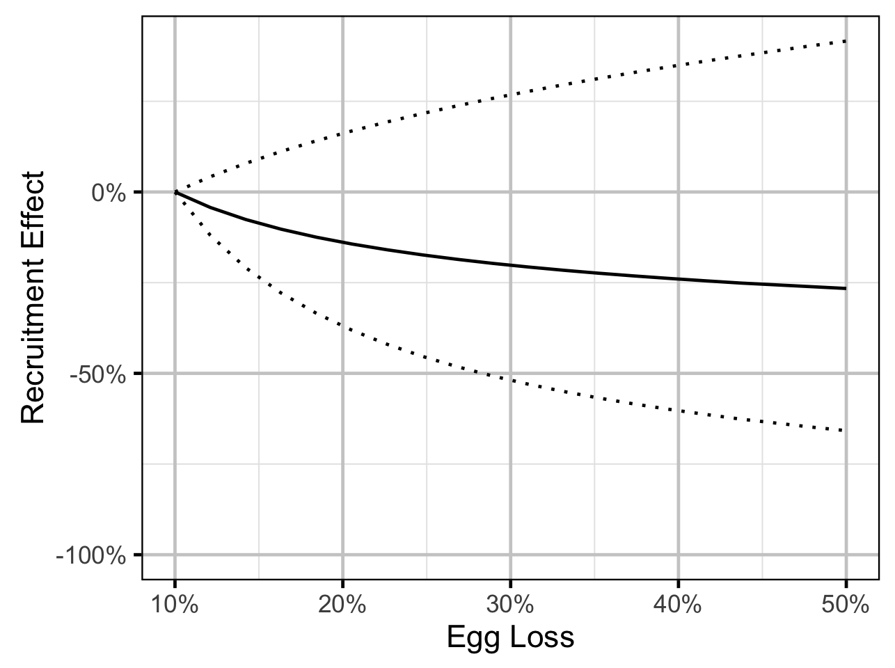
The relationship between percent dewatering and subsequent recruitment is expected to depend on stock abundance (Subbey et al. 2014) which might be changing over the course of the study. Consequently, preliminary analyses allowed the slope of the regression line to change by year. However, year was not a significant predictor and was therefore removed from the final model. The effect of dewatering on Mountain Whitefish abundance was expressed in terms of the predicted percent change in Age-1 Mountain Whitefish abundance by egg loss in the spawn year relative to 10% egg loss in the spawn year. The egg loss in the previous year was fixed at 10%. The percent change could not be calculated relative to 0% in the spawn or previous year as \(\Pi_t\) is undefined in either case.
Stock-Recruitment
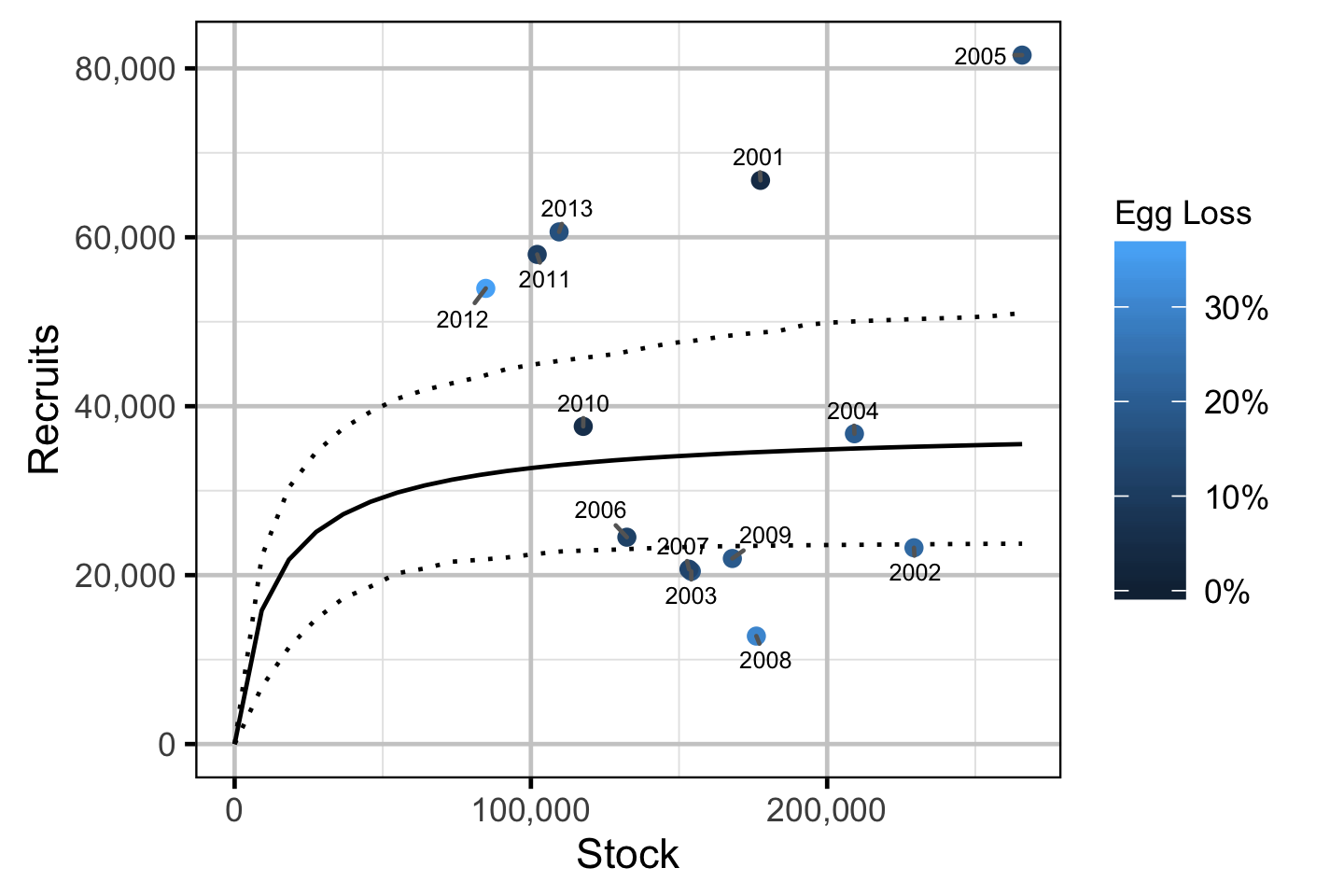
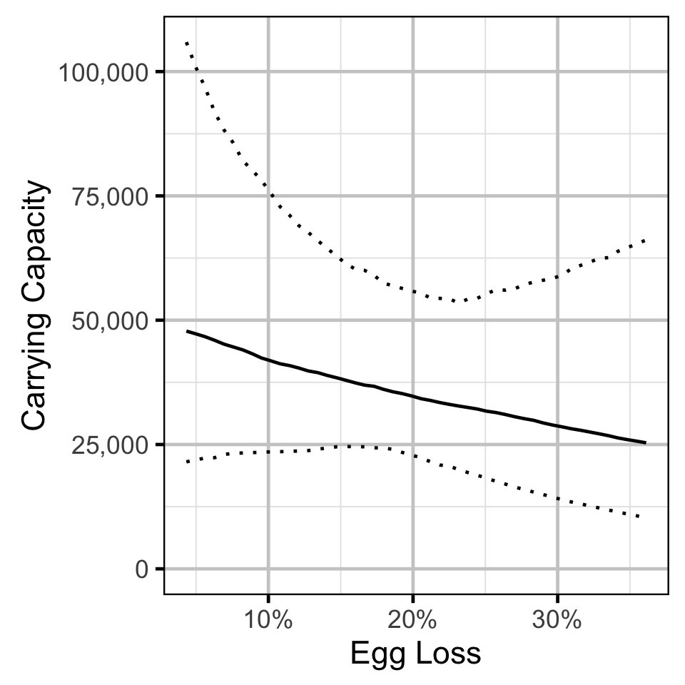
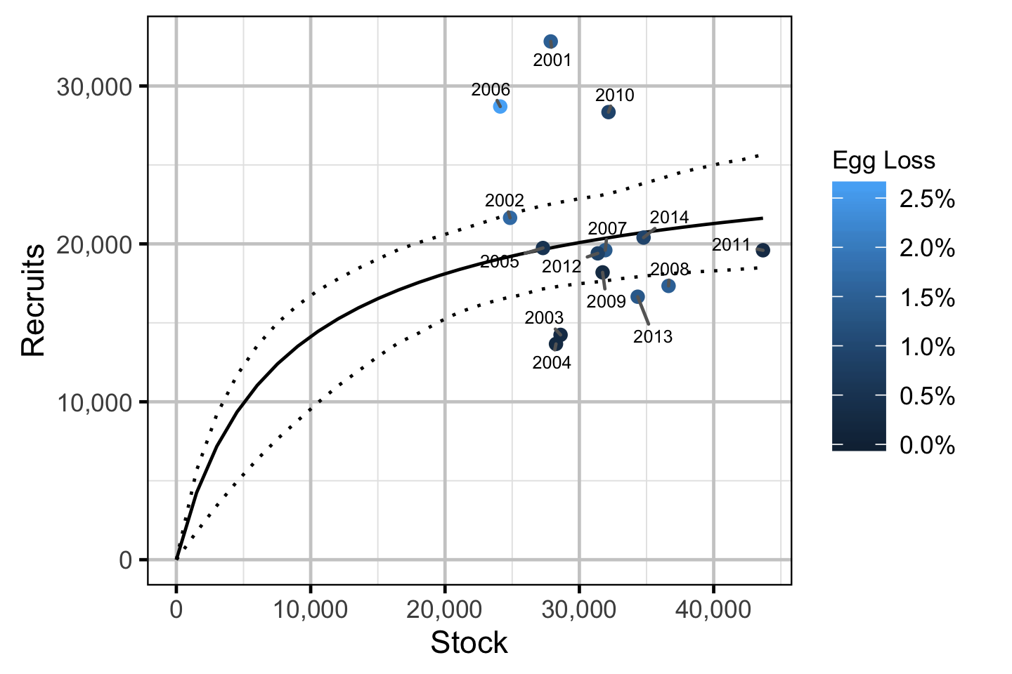
The relationship between the adults and the resultant number of age-1 subadultswas estimated using a Bayesian Beverton-Holt stock-recruitment model (Walters and Martell 2004):
\[ R = \frac{\alpha \cdot S}{1 + \beta \cdot S} \quad,\]
where \(S\) is the adults (stock), \(R\) is the subadults (recruits), \(\alpha\) is the recruits per spawner at low density and \(\beta\) determines the density-dependence.
Key assumptions of the stock-recruitment model include:
- The prior probability for \(\alpha\) is a uniform distribution from 0 to 5.
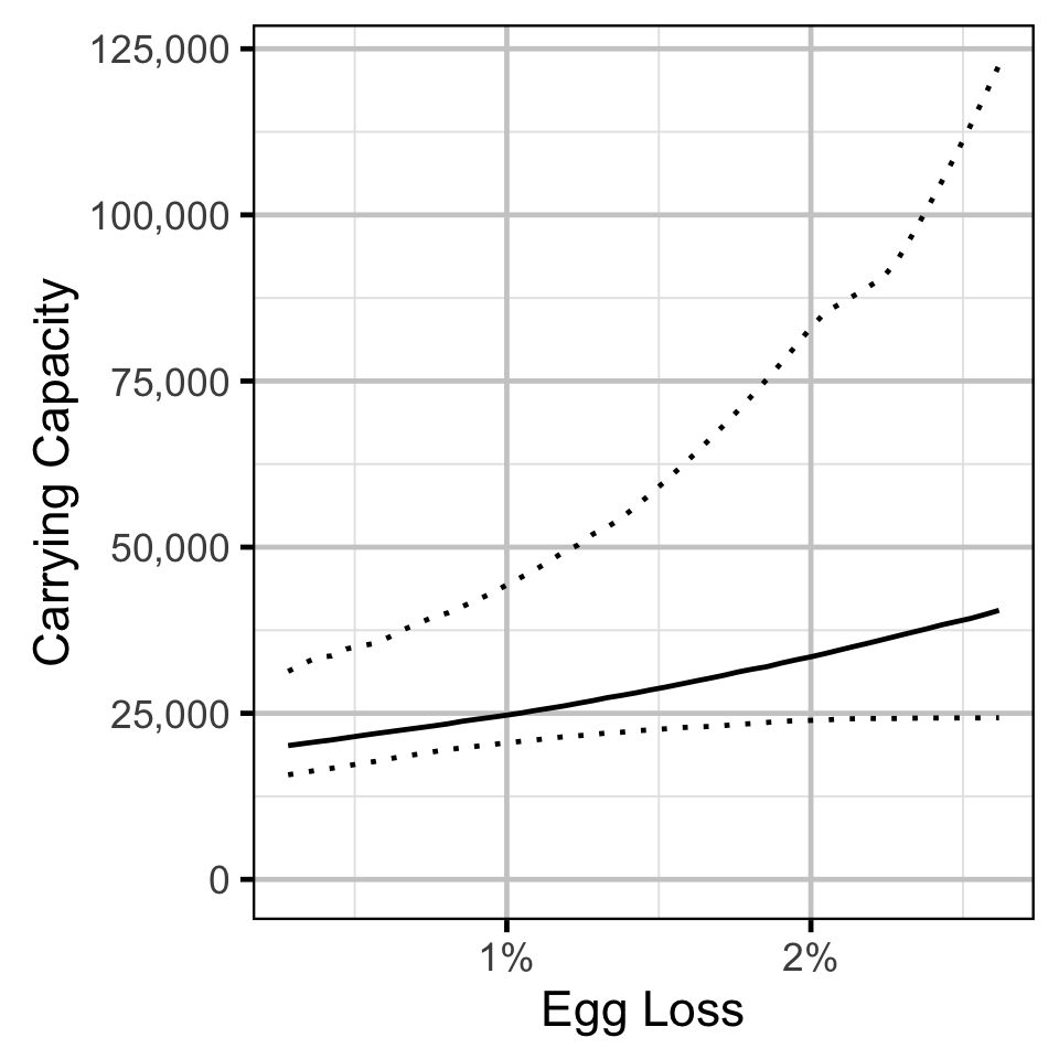
- The density-dependence varies with the proportional egg loss.
- The residual variation in the number of recruits is log-normally distributed.
The carrying capacity \(K\) is given by the relationship:
\[ K = \frac{\alpha}{\beta} \quad.\]
Model Code
The JAGS model code, which uses a series of naming conventions, is presented below.
Condition
| Variable/Parameter | Description |
|---|---|
bCorrelation |
Correlation coefficient between bWeightYear and bWeightLengthYear |
bWeight |
Intercept of eLogWeight |
bWeightDayte |
Linear effect of dayte on eLogWeight |
bWeightLength |
Linear effect of length on eLogWeight |
bWeightLengthDayte |
Effect of dayte on effect of length on eLogWeight |
bWeightLengthYear[i] |
Effect of ith year on effect of length on eLogWeight |
bWeightYear[i] |
Effect of ith year on eLogWeight |
Dayte[i] |
Day of year ith fish was captured |
eLogWeight[i] |
Expected log(Weight) of ith fish |
Length[i] |
log(Length) of ith fish |
sWeight |
SD of residual variation in log(Weight) |
sWeightLengthYear |
SD of effect of year on effect of length on eLogWeight |
sWeightYear |
SD of effect of year on eLogWeight |
Weight[i] |
Observed weight of ith fish |
Year[i] |
Year ith fish was captured |
Condition - Model1
model {

  bWeight ~ dnorm(5, 5^-2)
  bWeightLength ~ dnorm(3, 2^-2)

  bWeightDayte ~ dnorm(0, 2^-2)
  bWeightLengthDayte ~ dnorm(0, 2^-2)

  sWeightYear ~ dunif(0, 1)
  sWeightLengthYear ~ dunif(0, 1)
  for (i in 1:nYear) {
    bWeightYear[i] ~ dnorm(0, sWeightYear^-2)
    bWeightLengthYear[i] ~ dnorm(0, sWeightLengthYear^-2)
  }

  sWeight ~ dunif(0, 1)
  for(i in 1:length(Length)) {
    eLogWeight[i] <-    bWeight
                      + bWeightDayte * Dayte[i]
                      + bWeightYear[Year[i]]
                      + ( bWeightLength
                        + bWeightLengthDayte * Dayte[i]
                        + bWeightLengthYear[Year[i]]
                        ) * Length[i]

    Weight[i] ~ dlnorm(eLogWeight[i], sWeight^-2)
  }
}
Growth
| Variable/Parameter | Description |
|---|---|
bK |
Intercept of log(eK) |
bKYear[i] |
Random effect of ith year on log(eK) |
bLinf |
Mean maximum length |
eGrowth[i] |
Expected growth between release and recapture of ith recapture |
eK[i] |
Expected von Bertalanffy growth coefficient in ith year |
Growth[i] |
Observed growth between release and recapture of ith recapture |
LengthAtRelease[i] |
Length at previous release of ith recapture |
sGrowth |
SD of residual variation in Growth |
sKYear |
SD of effect of year on log(eK) |
Year[i] |
Release year of ith recapture |
Years[i] |
Years between release and recapture of ith recapture |
Growth - Model1
model {

  bK ~ dnorm (0, 5^-2)
  sKYear ~ dunif (0, 5)
  for (i in 1:nYear) {
    bKYear[i] ~ dnorm(0, sKYear^-2)
    log(eK[i]) <- bK + bKYear[i]
  }

  bLinf ~ dunif(100, 1000)
  sGrowth ~ dunif(0, 100)

  for (i in 1:length(Year)) {
    eGrowth[i] <- (bLinf - LengthAtRelease[i]) * (1 - exp(-sum(eK[Year[i]:(Year[i] + Years[i] - 1)])))

    Growth[i] ~ dnorm(eGrowth[i], sGrowth^-2)
  }
}
Length-At-Age
| Variable/Parameter | Description |
|---|---|
Age[ii] |
Observed age-class of iith fish |
bAge[ii] |
Effect of iith age-class on logit(pAgeYear) |
bAgeYear[ii, jj] |
Effect of iith age-class within jjth year on logit(pAgeYear) |
bDayte[ii] |
Effect of iith age-class on linear effect of dayte on eLength |
bDayte2[ii] |
Effect of iith age-class on quadratic effect of dayte on eLength |
bGrowthAge[ii] |
Growth of fish to iith age-class |
bGrowthAgeYear[ii, jj] |
Growth of fish to iith age-class within jjth year |
bLengthAgeYear[ii, jj] |
Effect of iith age-class within jjth year on eLength |
eGrowthAgeYear[ii, jj] |
Total growth of fish to iith age-class in jjth year |
eLength[ii] |
Expected length of iith fish |
Length[ii] |
Observed length of iith fish |
pAgeYear[ii, jj] |
Proportion of fish in iith age-class within jjth year |
sAgeYear |
SD of effect of age-class within year on bAgeYear |
sGrowthAgeYear[ii] |
SD of effect of age-class within year on fish growth |
sLengthAge[ii] |
SD of residual variation in eLength of fish in iith age-class |
Year[ii] |
Year in which iith fish was caught |
Length-At-Age - Model1
model{

  for(ii in 1:nAge){
    bGrowthAge[ii] ~ dunif(10, 100)
    sGrowthAgeYear[ii] ~ dunif(0, 25)
    for(jj in 1:nYear) {
      bGrowthAgeYear[ii, jj] ~ dnorm(0, sGrowthAgeYear[ii]^-2)
      eGrowthAgeYear[ii, jj] <- bGrowthAge[ii] + bGrowthAgeYear[ii, jj]
    }
  }

  bLengthAgeYear[1, 1] <- eGrowthAgeYear[1, 1]
  for(ii in 2:nAge){
    bLengthAgeYear[ii, 1] <- bLengthAgeYear[ii-1, 1] - bGrowthAgeYear[ii-1, 1] + eGrowthAgeYear[ii, 1]
  }

  for(jj in 2:nYear){
    bLengthAgeYear[1, jj] <- eGrowthAgeYear[1, jj]
    for(ii in 2:nAge){
      bLengthAgeYear[ii, jj] <- bLengthAgeYear[ii-1, jj-1] + eGrowthAgeYear[ii, jj]
    }
  }

  for(ii in 1:nAge)  {
    bDayte[ii] ~ dnorm(0, 10)
    bDayte2[ii] ~ dnorm(0, 10)
  }

  sAgeYear ~ dunif(0, 5)
  for(ii in 1:(nAge - 1)){
    bAge[ii] ~ dnorm(0, 2^-2)
    for(jj in 1:nYear){
      bAgeYear[ii, jj] ~ dnorm(0, sAgeYear^-2)
    }
  }

  for(jj in 1:nYear){
    logit(pAgeYear[1, jj]) <- bAge[1] + bAgeYear[1, jj]
    for(ii in 2:(nAge - 1)){
      pAgeYear[ii, jj] <- (1 - sum(pAgeYear[1:(ii - 1), jj])) * ilogit(bAge[ii] + bAgeYear[ii, jj])
    }
    pAgeYear[nAge, jj] <- (1 - sum(pAgeYear[1:(nAge - 1), jj]))
  }

    for(ii in 1:nAge){
    sLengthAge[ii] ~ dunif(0, 50)
  }

    for(ii in 1:length(Length)){
    Age[ii] ~ dcat(pAgeYear[1:nAge, Year[ii]])
    eLength[ii] <-  bLengthAgeYear[Age[ii], Year[ii]]
                  + bDayte[Age[ii]] * Dayte[ii]
                  + bDayte2[Age[ii]] * Dayte[ii]^2
    Length[ii] ~ dnorm(eLength[ii], sLengthAge[Age[ii]]^-2)
  }
}
Observer Length Correction
| Variable/Parameter | Description |
|---|---|
bLength[i] |
Relative inaccuracy of ith observer |
ClassLength[i] |
Mean length of fish belonging to ith class |
dClass[i] |
Prior value for the proportion of fish in the ith class |
eClass[i] |
Expected class of ith fish |
eLength[i] |
Expected length of ith fish |
eSLength[i] |
Expected SD of residual variation in length of ith fish |
Length[i] |
Observed fork length of ith fish |
Observer[i] |
Observer of ith fish where the first observer used a length board |
pClass[i] |
Proportion of fish in the ith class |
sLength[i] |
Relative imprecision of ith observer |
Year[i] |
Year ith fish was observed |
Observer Length Correction - Model1
model{

  for(j in 1:nYear){
    for(i in 1:nClass) {
      dClass[i, j] <- 1
    }
    pClass[1:nClass, j] ~ ddirch(dClass[, j])
  }

  bLength[1] <- 1
  sLength[1] <- 1

  for(i in 2:nObserver) {
    bLength[i] ~ dunif(0.5, 2)
    sLength[i] ~ dunif(2, 10)
  }

  for(i in 1:length(Length)){
    eClass[i] ~ dcat(pClass[, Year[i]])
    eLength[i] <- bLength[Observer[i]] * ClassLength[eClass[i]]
    eSLength[i] <- sLength[Observer[i]] * ClassSD
    Length[i] ~ dnorm(eLength[i], eSLength[i]^-2)
  }
}
Survival
| Variable/Parameter | Description |
|---|---|
bEfficiency |
Intercept for logit(eEfficiency) |
bEfficiencySampledLength |
Effect of SampledLength on bEfficiency |
bSurvival |
Intercept for logit(eSurvival) |
bSurvivalYear[i] |
Effect of Year on bSurvival |
eEfficiency[i] |
Expected recapture probability in ith year |
eSurvival[i] |
Expected survival probability from i-1th to ith year |
SampledLength |
Total standardised length of river sampled |
sSurvivalYear |
SD of bSurvivalYear |
Survival - Model1
model{
  bEfficiency ~ dnorm(0, 5^-2)
  bEfficiencySampledLength ~ dnorm(0, 5^-2)

  bSurvival ~ dnorm(0, 5^-2)

  sSurvivalYear ~ dunif(0, 5)
  for(i in 1:nYear) {
    bSurvivalYear[i] ~ dnorm(0, sSurvivalYear^-2)
  }

  for(i in 1:(nYear-1)) {
    logit(eEfficiency[i]) <- bEfficiency + bEfficiencySampledLength * SampledLength[i]
    logit(eSurvival[i]) <- bSurvival + bSurvivalYear[i]

    eProbability[i,i] <- eSurvival[i] * eEfficiency[i]
    for(j in (i+1):(nYear-1)) {
      eProbability[i,j] <- prod(eSurvival[i:j]) * prod(1-eEfficiency[i:(j-1)]) * eEfficiency[j]
    }
    for(j in 1:(i-1)) {
      eProbability[i,j] <- 0
    }
  }
  for(i in 1:(nYear-1)) {
    eProbability[i,nYear] <- 1 - sum(eProbability[i,1:(nYear-1)])
  }

  for(i in 1:(nYear - 1)) {
    Marray[i, 1:nYear] ~ dmulti(eProbability[i,], Released[i])
  }
}
Site Fidelity
| Variable/Parameter | Description |
|---|---|
bFidelity |
Intercept of logit(eFidelity) |
bLength |
Effect of length on logit(eFidelity) |
eFidelity[i] |
Expected site fidelity of ith recapture |
Fidelity[i] |
Whether the ith recapture was encountered at the same site as the previous encounter |
Length[i] |
Length at previous encounter of ith recapture |
Site Fidelity - Model1
model {

  bFidelity ~ dnorm(0, 2^-2)
  bLength ~ dnorm(0, 2^-2)

  for (i in 1:length(Fidelity)) {
    logit(eFidelity[i]) <- bFidelity + bLength * Length[i]
    Fidelity[i] ~ dbern(eFidelity[i])
  }
}
Capture Efficiency
| Variable/Parameter | Description |
|---|---|
bEfficiency |
Intercept for logit(eEfficiency) |
bEfficiencySessionYear |
Effect of Session within Year on logit(eEfficiency) |
eEfficiency[i] |
Expected efficiency on ith visit |
eFidelity[i] |
Expected site fidelity on ith visit |
Fidelity[i] |
Mean site fidelity on ith visit |
FidelitySD[i] |
SD of site fidelity on ith visit |
Recaptures[i] |
Number of marked fish recaught during ith visit |
sEfficiencySessionYear |
SD of effect of Session within Year on logit(eEfficiency) |
Session[i] |
Session of ith visit |
Tagged[i] |
Number of marked fish tagged prior to ith visit |
Year[i] |
Year of ith visit |
Capture Efficiency - Model1
model {

  bEfficiency ~ dnorm(0, 5^-2)

  sEfficiencySessionYear ~ dunif(0, 2)
  for (i in 1:nSession) {
    for (j in 1:nYear) {
      bEfficiencySessionYear[i, j] ~ dnorm(0, sEfficiencySessionYear^-2)
    }
  }

  for (i in 1:length(Recaptures)) {

    logit(eEfficiency[i]) <- bEfficiency + bEfficiencySessionYear[Session[i], Year[i]]

    eFidelity[i] ~ dnorm(Fidelity[i], FidelitySD[i]^-2) T(0, 1)
    Recaptures[i] ~ dbin(eEfficiency[i] * eFidelity[i], Tagged[i])
  }
}
Abundance
| Variable/Parameter | Description |
|---|---|
bDensity |
Intercept for log(eDensity) |
bDensitySite |
Effect of Site on log(eDensity) |
bDensitySiteYear |
Effect of Site within Year on log(eDensity) |
bDensityYear |
Effect of Year on log(eDensity) |
bVisitType |
Effect of VisitType on Efficiency |
eDensity[i] |
Expected density during ith visit |
eDispersion |
Overdispersion of Fish |
Efficiency[i] |
Survey efficiency during ith visit |
Fish[i] |
Observed count during ith visit |
ProportionSampled[i] |
Proportion of site surveyed during ith visit |
sDensitySite |
SD of effect of Site on log(eDensity) |
sDensitySiteYear |
SD of effect of Site within Year on log(eDensity) |
sDensityYear |
SD of effect of Year on log(eDensity) |
sDispersion |
SD of overdispersion term |
Site[i] |
Site of ith visit |
SiteLength[i] |
Length of site during ith visit |
VisitType[i] |
Survey type (catch versus count) during ith visit |
Year[i] |
Year of ith visit |
Abundance - Model1
model {
  bDensity ~ dnorm(5, 5^-2)

  bVisitType[1] <- 1
  for (i in 2:nVisitType) {
    bVisitType[i] ~ dunif(0, 10)
  }

  sDensityYear ~ dunif(0, 2)
  for (i in 1:nYear) {
    bDensityYear[i] ~ dnorm(0, sDensityYear^-2)
  }

  sDensitySite ~ dunif(0, 2)
  sDensitySiteYear ~ dunif(0, 2)
  for (i in 1:nSite) {
    bDensitySite[i] ~ dnorm(0, sDensitySite^-2)
    for (j in 1:nYear) {
      bDensitySiteYear[i, j] ~ dnorm(0, sDensitySiteYear^-2)
    }
  }

  sDispersion ~ dunif(0, 5)
  for (i in 1:length(Fish)) {
    log(eDensity[i]) <- bDensity + bDensitySite[Site[i]] + bDensityYear[Year[i]] + bDensitySiteYear[Site[i],Year[i]]

    eDispersion[i] ~ dgamma(1 / sDispersion^2, 1 / sDispersion^2)
    Fish[i] ~ dpois(eDensity[i] * SiteLength[i] * ProportionSampled[i] * Efficiency[i] * bVisitType[VisitType[i]] * eDispersion[i])
  }
}
Long-Term Trends
| Variable/Parameter | Description |
|---|---|
bDistance[i,j] |
Euclidean distance between ith and jth Variable |
bTrendYear[t,y] |
Expected value for tth trend in yth Year |
eValue[v,y,t] |
Expected standardised value for vth Variable in yth Year considering tth trends |
sTrend |
SD in trend random walks |
sValue |
SD for residual variation in Value |
Value[i] |
Standardised value for ith data point |
Variable[i] |
Variable for ith data point |
Year[i] |
Year of ith data point |
Z[v,y] |
Expected weighting for vth Variable in yth Year |
Long-Term Trends - Model1
model{

  sTrend ~ dunif(0, 1)
  for (t in 1:nTrend) {
    bTrendYear[t,1] ~ dunif(-1,1)
    for(y in 2:nYear){
      bTrendYear[t,y] ~ dnorm(bTrendYear[t,y-1], sTrend^-2)
    }
  }

  for(v in 1:nVariable){
    for(t in 1:nTrend) {
      Z[v,t] ~ dunif(-1,1)
    }
    for(y in 1:nYear){
      eValue[v,y,1] <- Z[v,1] * bTrendYear[1,y]
      for(t in 2:nTrend) {
        eValue[v,y,t] <- eValue[v,y,t-1] + Z[v,t] * bTrendYear[t,y]
      }
    }
  }

  sValue ~ dunif(0, 1)
  for(i in 1:length(Value)) {
    Value[i] ~ dnorm(eValue[Variable[i], Year[i], nTrend], sValue^-2)
  }

  for(i in 1:nVariable) {
    for(j in 1:nVariable) {
      bDistance[i,j] <- sqrt(sum((Z[i,]-Z[j,])^2))
    }
  }
}
Scale Age
| Variable/Parameter | Description |
|---|---|
Ager[i] |
ith ager |
bIntercept |
Intercept of eScaleAge |
bInterceptAger[i] |
Effect of Ager[i] on the intercept of eScaleAge |
bInterceptEncounterID[i] |
Random effect of EncounterID[i] on the intercept of eScaleAge |
bInterceptEncounterIDAger[i,j] |
Random effect of the interaction of EncounterID[i] and Ager[j] on the intercept of eScaleAge |
BirthYear[i] |
BirthYear of the ith fish |
bSlope |
Intercept on the slope of the effect of eAge on eScaleAge |
bSlopeAger[i] |
Effect of Ager[i] on the slope of the effect of eAge on eScaleAge |
dYear[i] |
ith parameter of the Dirichlet distribution on pYear |
eAge[i] |
Expected true age of the fish on the ith scale age observation |
EncounterID[i] |
ID of the ith encounter |
eScaleAge[i] |
Expected scale age on the ith scale age observation |
FishID[i] |
Fish ID of the ith scale age |
pYear[i] |
Probability that a fish is born in the ith year, starting with 1993 |
ScaleAge[i] |
ith scale age observation |
sInterceptEncounterID |
SD of bInterceptEncounterID |
sInterceptEncounterIDAger |
SD of bInterceptEncounterIDAger |
sSD[i] |
SD of the ith ager due to pseudo-replication |
Year[i] |
Encounter year of the ith scale age observation |
Scale Age - Model1
model {
  for(i in 1:nBirthYear) {
    dYear[i] <- 1
  }
  pYear ~ ddirch(dYear[])
  for(i in 1:nFishID){
    BirthYear[i] ~ dcat(pYear)
  }
  mBirthYear <- BirthYear
  bIntercept <- 0
  bSlope <- 1
  for(i in 1:nAger) {
    sSD[i] ~ dunif(0, 5)
  }
  for(i in 1:nAger) {
    bInterceptAger[i] ~ dnorm(0, 2^-2)
    bSlopeAger[i] ~ dnorm(0, 2^-2)
  }
  sInterceptEncounterID ~ dunif(0, 2)
  sInterceptEncounterIDAger ~ dunif(0, 2)
  for(i in 1:nEncounterID) {
    bInterceptEncounterID[i] ~ dnorm(0, sInterceptEncounterID^-2)
    for(j in 1:nAger) {
      bInterceptEncounterIDAger[i,j] ~ dnorm(0, sInterceptEncounterIDAger^-2)
    }
  }
  for(i in 1:length(ScaleAge)){
    eAge[i] <- Year[i] - BirthYear[FishID[i]]
    eScaleAge[i] <- bIntercept + bInterceptAger[Ager[i]] + (bSlope + bSlopeAger[Ager[i]]) * eAge[i] + bInterceptEncounterID[EncounterID[i]] + bInterceptEncounterIDAger[EncounterID[i], Ager[i]]
    ScaleAge[i] ~ dnorm(eScaleAge[i], sSD[Ager[i]]^-2) T(0,)
  }
}
Age-Ratios
| Variable/Parameter | Description |
|---|---|
Age1[i] |
The number of Age-1 fish in the ith year |
Age1and2[i] |
The number of Age-1 and Age-2 fish in the ith year |
bProbAge1 |
Intercept for logit(eProbAge1) |
bProbAge1Loss |
Effect of LossLogRatio on bProbAge1 |
eProbAge1[i] |
The expected proportion of Age-1 fish in the ith year |
LossLogRatio[i] |
The log of the ratio of the percent egg losses |
sDispersion |
SD of extra-binomial variation |
Age-Ratios - Model1
model{

  bProbAge1 ~ dnorm(0, 1000^-2)
  bProbAge1Loss ~ dnorm(0, 1000^-2)

  sDispersion ~ dunif(0, 1000)
  for(i in 1:length(LossLogRatio)){
    eDispersion[i] ~ dnorm(0, sDispersion^-2)
    logit(eProbAge1[i]) <- bProbAge1 + bProbAge1Loss * LossLogRatio[i] + eDispersion[i]
    Age1[i] ~ dbin(eProbAge1[i], Age1and2[i])
  }
}
Stock-Recruitment
| Variable/Parameter | Description |
|---|---|
bAlpha |
eRecruits per Stock at low Stock density |
bBeta |
Intercept for log(eBeta) |
bBetaEggLoss |
Effect of EggLoss on bBeta |
eBeta |
Effect of density-dependence |
EggLoss[i] |
Calculated proportional egg loss for ith spawn year |
eRecruits[i] |
Expected value of Recruits |
Recruits[i] |
Number of Age-1 recruits from ith spawn year |
sRecruits |
SD of residual variation in Recruits |
Stock[i] |
Number of Age-2+ spawners in ith spawn year |
Stock-Recruitment - Model1
model {

  bAlpha ~ dunif(0, 5)
  bBeta ~ dunif(0, 1)
  bBetaEggLoss ~ dnorm(0, 2^-2)

  sRecruits ~ dunif(0, 5)
  for(i in 1:length(Stock)){
    log(eBeta[i]) <- log(bBeta) + bBetaEggLoss * EggLoss[i]
    eRecruits[i] <- (bAlpha * Stock[i]) / (1 + eBeta[i] * Stock[i])
    Recruits[i] ~ dlnorm(log(eRecruits[i]), sRecruits^-2)
  }
}
Results
Model Parameters
The posterior distributions for the fixed (Kery and Schaub 2011 p. 75) parameters in each model are summarised below.
Condition - Mountain Whitefish
| Parameter | Estimate | Lower | Upper | SD | Error | Significance |
|---|---|---|---|---|---|---|
| bWeight | 5.424370 | 5.406310 | 5.445060 | 0.009990 | 0 | 0.0010 |
| bWeightDayte | -0.015066 | -0.019090 | -0.010863 | 0.002134 | 27 | 0.0010 |
| bWeightLength | 3.160900 | 3.107500 | 3.218900 | 0.029300 | 2 | 0.0010 |
| bWeightLengthDayte | -0.005500 | -0.016540 | 0.005660 | 0.005790 | 200 | 0.3474 |
| sWeight | 0.154752 | 0.152997 | 0.156710 | 0.000956 | 1 | 0.0010 |
| sWeightLengthYear | 0.111160 | 0.075100 | 0.168110 | 0.023690 | 42 | 0.0010 |
| sWeightYear | 0.045810 | 0.032460 | 0.066240 | 0.008920 | 37 | 0.0010 |
| Convergence | Iterations |
|---|---|
| 1.02 | 10000 |
Condition - Rainbow Trout
| Parameter | Estimate | Lower | Upper | SD | Error | Significance |
|---|---|---|---|---|---|---|
| bWeight | 5.952320 | 5.942210 | 5.963430 | 0.005420 | 0 | 0.001 |
| bWeightDayte | -0.003453 | -0.006563 | -0.000413 | 0.001526 | 89 | 0.028 |
| bWeightLength | 2.929740 | 2.899100 | 2.957610 | 0.014300 | 1 | 0.001 |
| bWeightLengthDayte | 0.044650 | 0.035310 | 0.053560 | 0.004710 | 20 | 0.001 |
| sWeight | 0.111289 | 0.109906 | 0.112719 | 0.000742 | 1 | 0.001 |
| sWeightLengthYear | 0.058340 | 0.037510 | 0.087850 | 0.013370 | 43 | 0.001 |
| sWeightYear | 0.024720 | 0.017140 | 0.035690 | 0.004750 | 38 | 0.001 |
| Convergence | Iterations |
|---|---|
| 1.04 | 10000 |
Condition - Walleye
| Parameter | Estimate | Lower | Upper | SD | Error | Significance |
|---|---|---|---|---|---|---|
| bWeight | 6.287860 | 6.265450 | 6.306010 | 0.009850 | 0 | 0.0010 |
| bWeightDayte | 0.018084 | 0.014997 | 0.021211 | 0.001611 | 17 | 0.0010 |
| bWeightLength | 3.220100 | 3.171200 | 3.273900 | 0.025500 | 2 | 0.0010 |
| bWeightLengthDayte | -0.014000 | -0.032850 | 0.005420 | 0.009550 | 140 | 0.1358 |
| sWeight | 0.098755 | 0.097282 | 0.100400 | 0.000796 | 2 | 0.0010 |
| sWeightLengthYear | 0.099390 | 0.064490 | 0.148790 | 0.022730 | 42 | 0.0010 |
| sWeightYear | 0.040760 | 0.029420 | 0.059710 | 0.008060 | 37 | 0.0010 |
| Convergence | Iterations |
|---|---|
| 1.04 | 10000 |
Growth - Mountain Whitefish
| Parameter | Estimate | Lower | Upper | SD | Error | Significance |
|---|---|---|---|---|---|---|
| bK | -1.1810 | -1.5232 | -0.9085 | 0.1523 | 26 | 7e-04 |
| bLinf | 407.9200 | 401.9800 | 414.2400 | 3.1400 | 2 | 7e-04 |
| sGrowth | 12.7340 | 11.4840 | 14.1220 | 0.6500 | 10 | 7e-04 |
| sKYear | 0.4573 | 0.2529 | 0.8177 | 0.1500 | 62 | 7e-04 |
| Convergence | Iterations |
|---|---|
| 1.06 | 4000 |
Growth - Rainbow Trout
| Parameter | Estimate | Lower | Upper | SD | Error | Significance |
|---|---|---|---|---|---|---|
| bK | -0.2041 | -0.3243 | -0.0812 | 0.0646 | 60 | 0.0014 |
| bLinf | 498.5600 | 493.6400 | 504.1000 | 2.6700 | 1 | 0.0007 |
| sGrowth | 29.7660 | 28.3510 | 31.1880 | 0.7130 | 5 | 0.0007 |
| sKYear | 0.2434 | 0.1636 | 0.3808 | 0.0539 | 45 | 0.0007 |
| Convergence | Iterations |
|---|---|
| 1.02 | 1000 |
Growth - Walleye
| Parameter | Estimate | Lower | Upper | SD | Error | Significance |
|---|---|---|---|---|---|---|
| bK | -2.8036 | -3.1421 | -2.4763 | 0.1744 | 12 | 7e-04 |
| bLinf | 867.3000 | 729.4000 | 988.3000 | 68.3000 | 15 | 7e-04 |
| sGrowth | 18.8670 | 17.3310 | 20.5080 | 0.8170 | 8 | 7e-04 |
| sKYear | 0.3275 | 0.1794 | 0.5432 | 0.0958 | 56 | 7e-04 |
| Convergence | Iterations |
|---|---|
| 1.04 | 2000 |
Length-At-Age - Mountain Whitefish
| Parameter | Estimate | Lower | Upper | SD | Error | Significance |
|---|---|---|---|---|---|---|
| bAge[1] | -1.9931 | -2.3632 | -1.6512 | 0.1848 | 18 | 0.0010 |
| bAge[2] | -0.8471 | -1.2793 | -0.4283 | 0.2229 | 50 | 0.0010 |
| bDayte[1] | 3.0928 | 2.6095 | 3.6037 | 0.2564 | 16 | 0.0010 |
| bDayte[2] | 2.4010 | 1.8910 | 2.9330 | 0.2650 | 22 | 0.0010 |
| bDayte[3] | 1.4300 | 0.8740 | 1.9820 | 0.2830 | 39 | 0.0010 |
| bDayte2[1] | -0.6846 | -1.1276 | -0.2755 | 0.2109 | 62 | 0.0010 |
| bDayte2[2] | -0.0914 | -0.4785 | 0.3162 | 0.2026 | 440 | 0.6867 |
| bDayte2[3] | 1.2020 | 0.6710 | 1.7260 | 0.2740 | 44 | 0.0010 |
| bGrowthAge[1] | 99.0810 | 97.3210 | 99.9780 | 0.7770 | 1 | 0.0010 |
| bGrowthAge[2] | 96.7060 | 93.0080 | 99.6640 | 1.8550 | 3 | 0.0010 |
| bGrowthAge[3] | 98.9240 | 96.2030 | 99.9730 | 1.0180 | 2 | 0.0010 |
| sAgeYear | 0.8713 | 0.6665 | 1.1408 | 0.1204 | 27 | 0.0010 |
| sGrowthAgeYear[1] | 22.2950 | 17.6960 | 24.8810 | 1.9610 | 16 | 0.0010 |
| sGrowthAgeYear[2] | 9.6290 | 6.4100 | 14.4900 | 2.1170 | 42 | 0.0010 |
| sGrowthAgeYear[3] | 23.7380 | 21.0460 | 24.9500 | 1.0710 | 8 | 0.0010 |
| sLengthAge[1] | 14.4989 | 14.1175 | 14.8843 | 0.2021 | 3 | 0.0010 |
| sLengthAge[2] | 21.9360 | 21.1250 | 22.7830 | 0.4180 | 4 | 0.0010 |
| sLengthAge[3] | 45.4510 | 44.6890 | 46.2240 | 0.3870 | 2 | 0.0010 |
| Convergence | Iterations |
|---|---|
| 1.05 | 10000 |
Length-At-Age - Rainbow Trout
| Parameter | Estimate | Lower | Upper | SD | Error | Significance |
|---|---|---|---|---|---|---|
| bAge[1] | -3.1540 | -3.4546 | -2.8313 | 0.1585 | 10 | 0.0010 |
| bAge[2] | 0.4468 | 0.2107 | 0.7704 | 0.1430 | 63 | 0.0040 |
| bDayte[1] | 0.8170 | 0.2620 | 1.3920 | 0.2970 | 69 | 0.0040 |
| bDayte[2] | 3.0350 | 2.5060 | 3.5450 | 0.2670 | 17 | 0.0010 |
| bDayte[3] | 0.2790 | -0.3330 | 0.9060 | 0.3060 | 220 | 0.3593 |
| bDayte2[1] | 0.0490 | -0.4900 | 0.5710 | 0.2750 | 1100 | 0.8743 |
| bDayte2[2] | 0.7356 | 0.2526 | 1.2048 | 0.2362 | 65 | 0.0020 |
| bDayte2[3] | 0.3450 | -0.1760 | 0.8840 | 0.2730 | 150 | 0.2016 |
| bGrowthAge[1] | 99.0050 | 96.3850 | 99.9690 | 0.9630 | 2 | 0.0010 |
| bGrowthAge[2] | 99.4760 | 97.8960 | 99.9810 | 0.5340 | 1 | 0.0010 |
| bGrowthAge[3] | 99.5270 | 98.2050 | 99.9880 | 0.4580 | 1 | 0.0010 |
| sAgeYear | 0.6505 | 0.4979 | 0.8472 | 0.0918 | 27 | 0.0010 |
| sGrowthAgeYear[1] | 19.4600 | 14.0400 | 24.5200 | 2.8200 | 27 | 0.0010 |
| sGrowthAgeYear[2] | 24.6960 | 23.9450 | 24.9920 | 0.2780 | 2 | 0.0010 |
| sGrowthAgeYear[3] | 24.8295 | 24.3591 | 24.9956 | 0.1677 | 1 | 0.0010 |
| sLengthAge[1] | 18.1640 | 17.2610 | 19.1650 | 0.4840 | 5 | 0.0010 |
| sLengthAge[2] | 38.1550 | 37.4970 | 38.7840 | 0.3340 | 2 | 0.0010 |
| sLengthAge[3] | 49.9275 | 49.7136 | 49.9984 | 0.0727 | 0 | 0.0010 |
| Convergence | Iterations |
|---|---|
| 1.03 | 10000 |
Observer Length Correction - Mountain Whitefish
| Parameter | Estimate | Lower | Upper | SD | Error | Significance |
|---|---|---|---|---|---|---|
| bLength[1] | 1.00000 | 1.00000 | 1.00000 | 0.00000 | 0 | 0.001 |
| bLength[2] | 0.91427 | 0.90470 | 0.92417 | 0.00500 | 1 | 0.001 |
| bLength[3] | 0.86202 | 0.85032 | 0.87484 | 0.00629 | 1 | 0.001 |
| bLength[4] | 0.86742 | 0.83560 | 0.89047 | 0.01323 | 3 | 0.001 |
| bLength[5] | 0.88006 | 0.87199 | 0.88733 | 0.00391 | 1 | 0.001 |
| sLength[1] | 1.00000 | 1.00000 | 1.00000 | 0.00000 | 0 | 0.001 |
| sLength[2] | 2.02053 | 2.00062 | 2.07767 | 0.02047 | 2 | 0.001 |
| sLength[3] | 3.69060 | 3.27810 | 4.13140 | 0.22320 | 12 | 0.001 |
| sLength[4] | 2.02970 | 2.00070 | 2.11350 | 0.03080 | 3 | 0.001 |
| sLength[5] | 2.00622 | 2.00017 | 2.02330 | 0.00629 | 1 | 0.001 |
| Convergence | Iterations |
|---|---|
| 1.02 | 10000 |
Observer Length Correction - Rainbow Trout
| Parameter | Estimate | Lower | Upper | SD | Error | Significance |
|---|---|---|---|---|---|---|
| bLength[1] | 1.00000 | 1.00000 | 1.00000 | 0.00000 | 0 | 0.001 |
| bLength[2] | 0.85658 | 0.84843 | 0.86427 | 0.00416 | 1 | 0.001 |
| bLength[3] | 0.86109 | 0.85000 | 0.87311 | 0.00585 | 1 | 0.001 |
| bLength[4] | 0.76364 | 0.73892 | 0.78866 | 0.01271 | 3 | 0.001 |
| bLength[5] | 0.85534 | 0.84924 | 0.86174 | 0.00316 | 1 | 0.001 |
| sLength[1] | 1.00000 | 1.00000 | 1.00000 | 0.00000 | 0 | 0.001 |
| sLength[2] | 2.02375 | 2.00076 | 2.08957 | 0.02432 | 2 | 0.001 |
| sLength[3] | 2.57100 | 2.02700 | 3.28500 | 0.34200 | 24 | 0.001 |
| sLength[4] | 4.40400 | 3.12200 | 5.88400 | 0.68600 | 31 | 0.001 |
| sLength[5] | 2.01610 | 2.00031 | 2.05944 | 0.01643 | 1 | 0.001 |
| Convergence | Iterations |
|---|---|
| 1.04 | 10000 |
Observer Length Correction - Walleye
| Parameter | Estimate | Lower | Upper | SD | Error | Significance |
|---|---|---|---|---|---|---|
| bLength[1] | 1.00000 | 1.00000 | 1.00000 | 0.00000 | 0 | 0.001 |
| bLength[2] | 0.80463 | 0.77794 | 0.84193 | 0.01706 | 4 | 0.001 |
| bLength[3] | 0.91895 | 0.90352 | 0.93395 | 0.00799 | 2 | 0.001 |
| bLength[4] | 0.85273 | 0.82315 | 0.89489 | 0.01820 | 4 | 0.001 |
| bLength[5] | 0.93104 | 0.91736 | 0.94542 | 0.00737 | 2 | 0.001 |
| sLength[1] | 1.00000 | 1.00000 | 1.00000 | 0.00000 | 0 | 0.001 |
| sLength[2] | 3.50600 | 2.02100 | 5.90800 | 1.26400 | 55 | 0.001 |
| sLength[3] | 2.54500 | 2.01300 | 4.38400 | 0.59300 | 47 | 0.001 |
| sLength[4] | 2.80700 | 2.01400 | 4.94200 | 0.83200 | 52 | 0.001 |
| sLength[5] | 2.12420 | 2.00230 | 2.52730 | 0.16570 | 12 | 0.001 |
| Convergence | Iterations |
|---|---|
| 1.06 | 10000 |
Survival - Mountain Whitefish
| Parameter | Estimate | Lower | Upper | SD | Error | Significance |
|---|---|---|---|---|---|---|
| bEfficiency | -4.7426 | -4.9714 | -4.4943 | 0.1237 | 5 | 0.0010 |
| bEfficiencySampledLength | 0.3685 | 0.1123 | 0.6191 | 0.1331 | 69 | 0.0080 |
| bSurvival | 0.5120 | -0.2480 | 1.5780 | 0.4420 | 180 | 0.1897 |
| sSurvivalYear | 1.4220 | 0.6820 | 2.7070 | 0.5310 | 71 | 0.0010 |
| Convergence | Iterations |
|---|---|
| 1.04 | 10000 |
Survival - Rainbow Trout
| Parameter | Estimate | Lower | Upper | SD | Error | Significance |
|---|---|---|---|---|---|---|
| bEfficiency | -3.1917 | -3.3926 | -2.9925 | 0.1052 | 6 | 0.0010 |
| bEfficiencySampledLength | 0.0171 | -0.1717 | 0.1904 | 0.0930 | 1100 | 0.8503 |
| bSurvival | -0.5470 | -0.8470 | -0.2489 | 0.1566 | 55 | 0.0020 |
| sSurvivalYear | 0.4188 | 0.1971 | 0.7474 | 0.1497 | 66 | 0.0010 |
| Convergence | Iterations |
|---|---|
| 1.01 | 10000 |
Survival - Walleye
| Parameter | Estimate | Lower | Upper | SD | Error | Significance |
|---|---|---|---|---|---|---|
| bEfficiency | -4.0380 | -4.2540 | -3.8131 | 0.1118 | 5 | 0.0010 |
| bEfficiencySampledLength | 0.0716 | -0.1053 | 0.2718 | 0.0967 | 260 | 0.4611 |
| bSurvival | -0.0143 | -0.3643 | 0.3912 | 0.1935 | 2600 | 0.9022 |
| sSurvivalYear | 0.5614 | 0.2347 | 1.1094 | 0.2152 | 78 | 0.0010 |
| Convergence | Iterations |
|---|---|
| 1.02 | 10000 |
Site Fidelity - Mountain Whitefish
| Parameter | Estimate | Lower | Upper | SD | Error | Significance |
|---|---|---|---|---|---|---|
| bFidelity | -0.1591 | -0.5215 | 0.2092 | 0.1864 | 230 | 0.3960 |
| bLength | -0.1244 | -0.5324 | 0.2515 | 0.1979 | 320 | 0.5294 |
| Convergence | Iterations |
|---|---|
| 1 | 1000 |
Site Fidelity - Rainbow Trout
| Parameter | Estimate | Lower | Upper | SD | Error | Significance |
|---|---|---|---|---|---|---|
| bFidelity | 0.8356 | 0.6709 | 1.0041 | 0.0857 | 20 | 7e-04 |
| bLength | -0.3489 | -0.5189 | -0.1903 | 0.0826 | 47 | 7e-04 |
| Convergence | Iterations |
|---|---|
| 1.01 | 1000 |
Site Fidelity - Walleye
| Parameter | Estimate | Lower | Upper | SD | Error | Significance |
|---|---|---|---|---|---|---|
| bFidelity | 0.7068 | 0.4225 | 1.0060 | 0.1510 | 41 | 0.0007 |
| bLength | -0.0974 | -0.3909 | 0.1949 | 0.1497 | 300 | 0.5134 |
| Convergence | Iterations |
|---|---|
| 1.01 | 1000 |
Capture Efficiency - Mountain Whitefish - Subadult
| Parameter | Estimate | Lower | Upper | SD | Error | Significance |
|---|---|---|---|---|---|---|
| bEfficiency | -4.9651 | -5.4962 | -4.5578 | 0.2399 | 9 | 0.001 |
| sEfficiencySessionYear | 0.4570 | 0.0130 | 1.1490 | 0.3170 | 120 | 0.001 |
| Convergence | Iterations |
|---|---|
| 1.02 | 20000 |
Capture Efficiency - Mountain Whitefish - Adult
| Parameter | Estimate | Lower | Upper | SD | Error | Significance |
|---|---|---|---|---|---|---|
| bEfficiency | -5.1857 | -5.5147 | -4.9082 | 0.1536 | 6 | 0.001 |
| sEfficiencySessionYear | 0.2660 | 0.0373 | 0.6738 | 0.1681 | 120 | 0.001 |
| Convergence | Iterations |
|---|---|
| 1.06 | 10000 |
Capture Efficiency - Rainbow Trout - Subadult
| Parameter | Estimate | Lower | Upper | SD | Error | Significance |
|---|---|---|---|---|---|---|
| bEfficiency | -3.3595 | -3.4944 | -3.2360 | 0.0668 | 4 | 0.001 |
| sEfficiencySessionYear | 0.3888 | 0.2688 | 0.5243 | 0.0644 | 33 | 0.001 |
| Convergence | Iterations |
|---|---|
| 1.01 | 10000 |
Capture Efficiency - Rainbow Trout - Adult
| Parameter | Estimate | Lower | Upper | SD | Error | Significance |
|---|---|---|---|---|---|---|
| bEfficiency | -4.0582 | -4.2215 | -3.9124 | 0.0799 | 4 | 0.001 |
| sEfficiencySessionYear | 0.2203 | 0.0197 | 0.4396 | 0.1116 | 95 | 0.001 |
| Convergence | Iterations |
|---|---|
| 1.02 | 10000 |
Capture Efficiency - Walleye - Adult
| Parameter | Estimate | Lower | Upper | SD | Error | Significance |
|---|---|---|---|---|---|---|
| bEfficiency | -4.4631 | -4.6975 | -4.2344 | 0.1190 | 5 | 0.001 |
| sEfficiencySessionYear | 0.6125 | 0.4107 | 0.8769 | 0.1208 | 38 | 0.001 |
| Convergence | Iterations |
|---|---|
| 1.03 | 10000 |
Abundance - Mountain Whitefish - Subadult
| Parameter | Estimate | Lower | Upper | SD | Error | Significance |
|---|---|---|---|---|---|---|
| bDensity | 5.36470 | 5.00840 | 5.6595 | 0.17420 | 6 | 0.001 |
| bVisitType[1] | 1.00000 | 1.00000 | 1.0000 | 0.00000 | 0 | 0.001 |
| bVisitType[2] | 4.13100 | 3.54900 | 4.8370 | 0.33600 | 16 | 0.001 |
| sDensitySite | 0.81530 | 0.65470 | 1.0286 | 0.09420 | 23 | 0.001 |
| sDensitySiteYear | 0.46200 | 0.40170 | 0.5302 | 0.03210 | 14 | 0.001 |
| sDensityYear | 0.73410 | 0.50900 | 1.0830 | 0.15290 | 39 | 0.001 |
| sDispersion | 0.50023 | 0.45882 | 0.5413 | 0.02111 | 8 | 0.001 |
| Convergence | Iterations |
|---|---|
| 1.08 | 10000 |
Abundance - Mountain Whitefish - Adult
| Parameter | Estimate | Lower | Upper | SD | Error | Significance |
|---|---|---|---|---|---|---|
| bDensity | 6.46330 | 6.04450 | 6.72500 | 0.16700 | 5 | 0.001 |
| bVisitType[1] | 1.00000 | 1.00000 | 1.00000 | 0.00000 | 0 | 0.001 |
| bVisitType[2] | 4.91600 | 4.17200 | 5.76700 | 0.41500 | 16 | 0.001 |
| sDensitySite | 1.12670 | 0.91200 | 1.36630 | 0.11590 | 20 | 0.001 |
| sDensitySiteYear | 0.41310 | 0.36010 | 0.47010 | 0.02850 | 13 | 0.001 |
| sDensityYear | 0.39250 | 0.25270 | 0.63750 | 0.09320 | 49 | 0.001 |
| sDispersion | 0.53922 | 0.50833 | 0.57488 | 0.01679 | 6 | 0.001 |
| Convergence | Iterations |
|---|---|
| 1.05 | 20000 |
Abundance - Rainbow Trout - Subadult
| Parameter | Estimate | Lower | Upper | SD | Error | Significance |
|---|---|---|---|---|---|---|
| bDensity | 4.82630 | 4.55990 | 5.08550 | 0.13110 | 5 | 0.001 |
| bVisitType[1] | 1.00000 | 1.00000 | 1.00000 | 0.00000 | 0 | 0.001 |
| bVisitType[2] | 4.23200 | 3.75200 | 4.80700 | 0.27000 | 12 | 0.001 |
| sDensitySite | 0.75020 | 0.61290 | 0.92000 | 0.07860 | 20 | 0.001 |
| sDensitySiteYear | 0.40880 | 0.35920 | 0.45950 | 0.02580 | 12 | 0.001 |
| sDensityYear | 0.32360 | 0.20810 | 0.51060 | 0.08050 | 47 | 0.001 |
| sDispersion | 0.40328 | 0.37313 | 0.43576 | 0.01563 | 8 | 0.001 |
| Convergence | Iterations |
|---|---|
| 1.03 | 40000 |
Abundance - Rainbow Trout - Adult
| Parameter | Estimate | Lower | Upper | SD | Error | Significance |
|---|---|---|---|---|---|---|
| bDensity | 5.32330 | 5.07870 | 5.55360 | 0.11960 | 4 | 0.001 |
| bVisitType[1] | 1.00000 | 1.00000 | 1.00000 | 0.00000 | 0 | 0.001 |
| bVisitType[2] | 4.40500 | 3.88800 | 4.99000 | 0.27800 | 13 | 0.001 |
| sDensitySite | 0.68580 | 0.56070 | 0.82960 | 0.06980 | 20 | 0.001 |
| sDensitySiteYear | 0.25922 | 0.20764 | 0.30729 | 0.02545 | 19 | 0.001 |
| sDensityYear | 0.23530 | 0.14900 | 0.37430 | 0.05660 | 48 | 0.001 |
| sDispersion | 0.40359 | 0.36958 | 0.43821 | 0.01703 | 9 | 0.001 |
| Convergence | Iterations |
|---|---|
| 1.06 | 10000 |
Abundance - Walleye - Adult
| Parameter | Estimate | Lower | Upper | SD | Error | Significance |
|---|---|---|---|---|---|---|
| bDensity | 5.33400 | 5.03470 | 5.59550 | 0.14040 | 5 | 0.001 |
| bVisitType[1] | 1.00000 | 1.00000 | 1.00000 | 0.00000 | 0 | 0.001 |
| bVisitType[2] | 4.27900 | 3.64600 | 4.88500 | 0.31700 | 14 | 0.001 |
| sDensitySite | 0.37980 | 0.28170 | 0.50120 | 0.05560 | 29 | 0.001 |
| sDensitySiteYear | 0.23607 | 0.18586 | 0.28434 | 0.02567 | 21 | 0.001 |
| sDensityYear | 0.51690 | 0.34770 | 0.75250 | 0.10730 | 39 | 0.001 |
| sDispersion | 0.46160 | 0.43091 | 0.49239 | 0.01635 | 7 | 0.001 |
| Convergence | Iterations |
|---|---|
| 1.05 | 20000 |
Long-Term Trends
| Parameter | Estimate | Lower | Upper | SD | Error | Significance |
|---|---|---|---|---|---|---|
| sTrend | 0.3627 | 0.1898 | 0.5269 | 0.0842 | 46 | 0.001 |
| sValue | 0.7832 | 0.6920 | 0.8864 | 0.0522 | 12 | 0.001 |
| Convergence | Iterations |
|---|---|
| 1.04 | 10000 |
Scale Age
| Parameter | Estimate | Lower | Upper | SD | Error | Significance |
|---|---|---|---|---|---|---|
| bInterceptAger[1] | 1.29500 | 1.14760 | 1.42600 | 0.07170 | 11 | 0.0007 |
| bInterceptAger[2] | 1.12120 | 0.95820 | 1.26890 | 0.07640 | 14 | 0.0007 |
| bSlope | 1.00000 | 1.00000 | 1.00000 | 0.00000 | 0 | 0.0007 |
| bSlopeAger[1] | -0.09540 | -0.18970 | 0.00980 | 0.05000 | 100 | 0.0734 |
| bSlopeAger[2] | -0.13070 | -0.22330 | -0.02620 | 0.04950 | 75 | 0.0107 |
| sInterceptEncounterID | 0.31960 | 0.23610 | 0.39580 | 0.04040 | 25 | 0.0007 |
| sInterceptEncounterIDAger | 0.28830 | 0.19960 | 0.36750 | 0.04180 | 29 | 0.0007 |
| sSD[1] | 0.38032 | 0.34306 | 0.42143 | 0.02045 | 10 | 0.0007 |
| sSD[2] | 0.51450 | 0.46390 | 0.57300 | 0.02830 | 11 | 0.0007 |
| Convergence | Iterations |
|---|---|
| 1.04 | 8000 |
Age-Ratios
| Parameter | Estimate | Lower | Upper | SD | Error | Significance |
|---|---|---|---|---|---|---|
| bProbAge1 | 0.4956 | 0.1033 | 0.9015 | 0.2043 | 81 | 0.0243 |
| bProbAge1Loss | -0.2332 | -0.6662 | 0.2161 | 0.2247 | 190 | 0.2887 |
| sDispersion | 0.7075 | 0.4644 | 1.1017 | 0.1710 | 45 | 0.0010 |
| Convergence | Iterations |
|---|---|
| 1.04 | 5000 |
Stock-Recruitment - Mountain Whitefish
| Parameter | Estimate | Lower | Upper | SD | Error | Significance |
|---|---|---|---|---|---|---|
| bAlpha | 3.2990000 | 0.8770000 | 4.9300000 | 1.1600000 | 61 | 0.0010 |
| bBeta | 0.0000937 | 0.0000166 | 0.0001761 | 0.0000419 | 85 | 0.0010 |
| bBetaEggLoss | 0.1764000 | -0.2686000 | 0.6067000 | 0.2156000 | 250 | 0.3613 |
| sRecruits | 0.6691000 | 0.4395000 | 1.0678000 | 0.1675000 | 47 | 0.0010 |
| Convergence | Iterations |
|---|---|
| 1 | 10000 |
Stock-Recruitment - Rainbow Trout
| Parameter | Estimate | Lower | Upper | SD | Error | Significance |
|---|---|---|---|---|---|---|
| bAlpha | 3.4660000 | 1.2140000 | 4.9320000 | 1.0370000 | 54 | 0.001 |
| bBeta | 0.0001401 | 0.0000264 | 0.0002219 | 0.0000533 | 70 | 0.001 |
| bBetaEggLoss | -0.2141000 | -0.4867000 | -0.0095000 | 0.1228000 | 110 | 0.042 |
| sRecruits | 0.2487000 | 0.1652000 | 0.3943000 | 0.0586000 | 46 | 0.001 |
| Convergence | Iterations |
|---|---|
| 1.09 | 10000 |
Figures
Condition
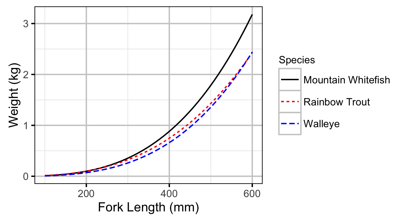
Condition - Mountain Whitefish - Subadult
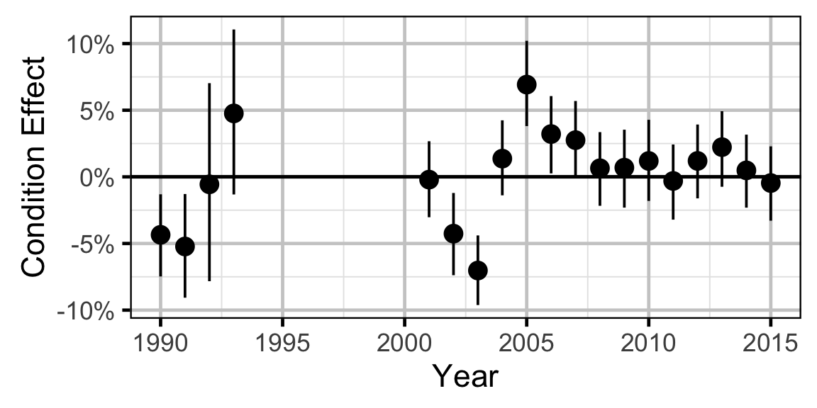
Condition - Mountain Whitefish - Adult
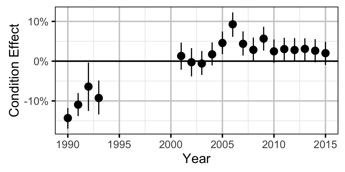
Condition - Rainbow Trout - Subadult
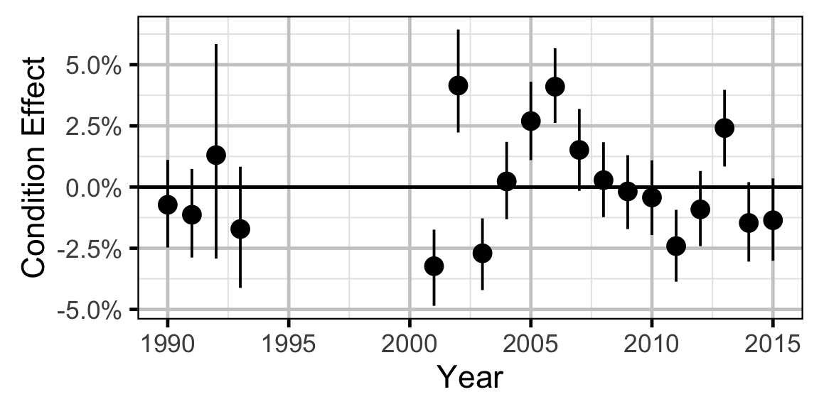
Condition - Rainbow Trout - Adult
Condition - Walleye - Adult
Growth
Growth - Mountain Whitefish
Growth - Rainbow Trout
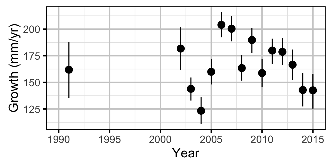
Growth - Walleye
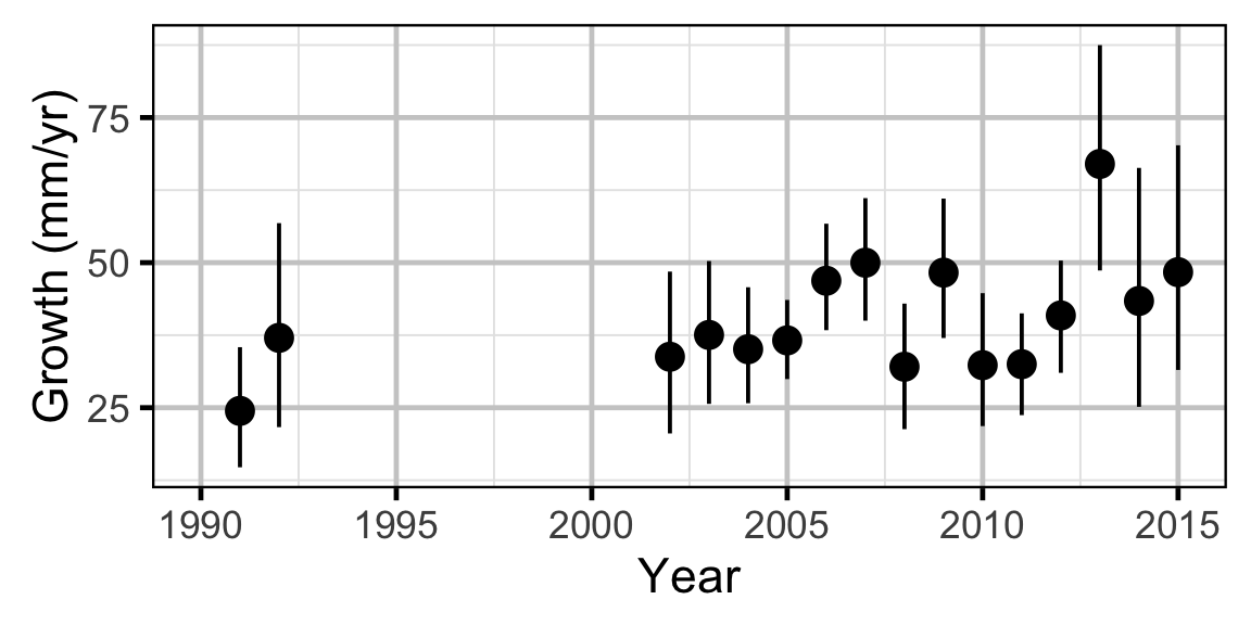
Length-At-Age - Mountain Whitefish
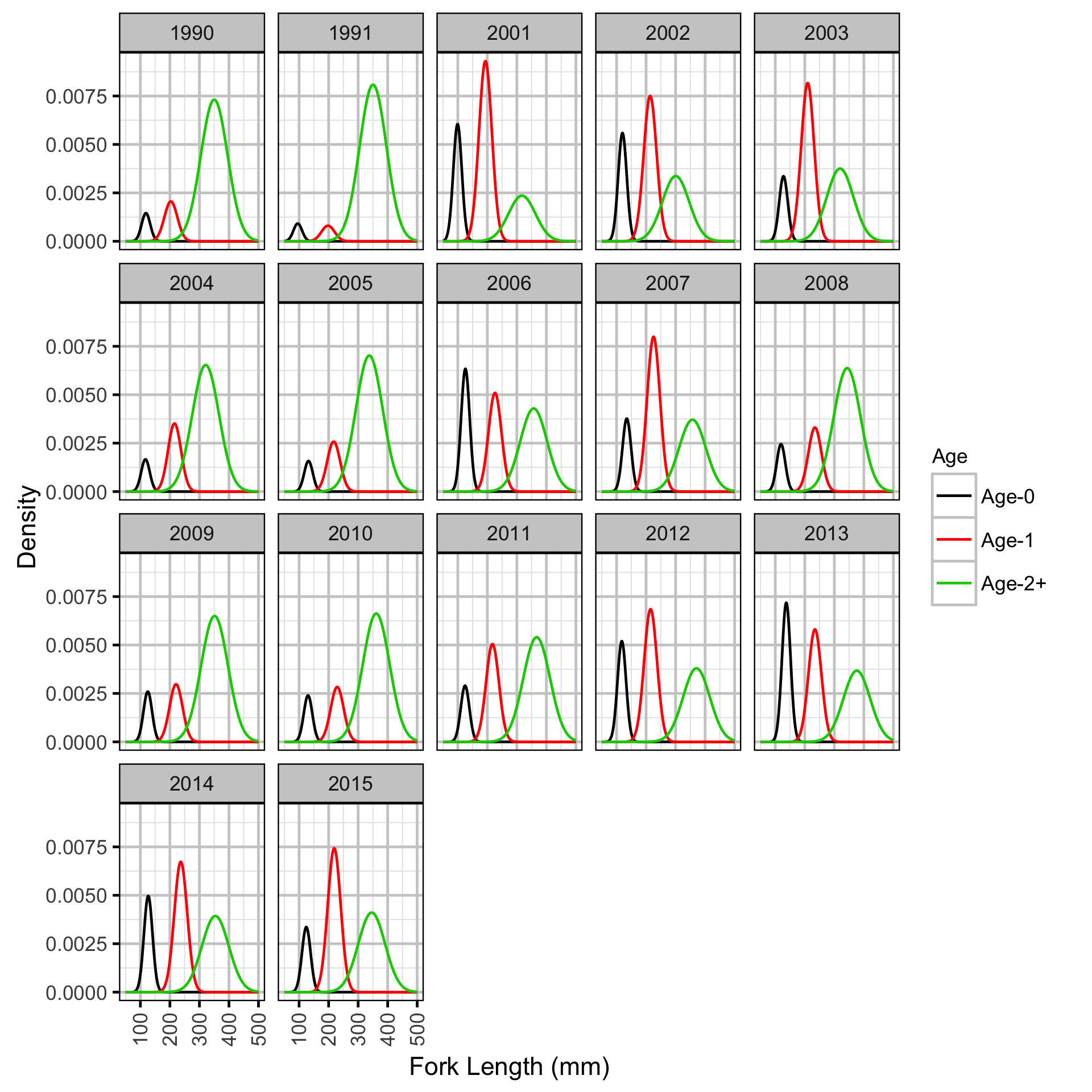
Length-At-Age - Mountain Whitefish - Age-0
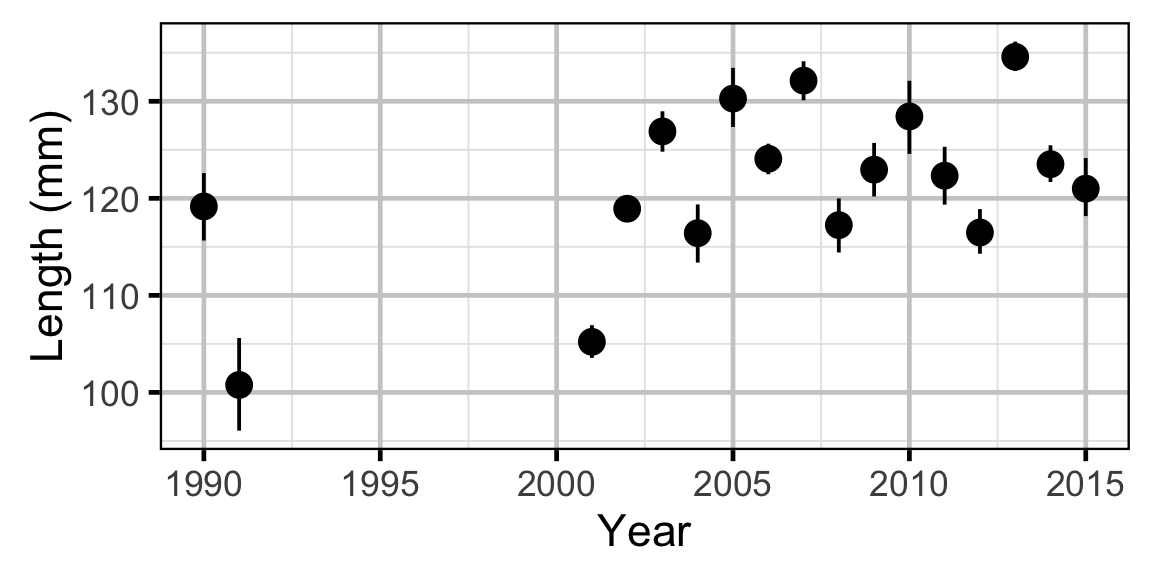
Length-At-Age - Mountain Whitefish - Age-1
Length-At-Age - Rainbow Trout
Length-At-Age - Rainbow Trout - Age-0
Length-At-Age - Rainbow Trout - Age-1
Observer Length Correction
Survival - Mountain Whitefish - Adult
Survival - Rainbow Trout - Adult
Survival - Walleye - Adult
Site Fidelity
Capture Efficiency
Capture Efficiency - Mountain Whitefish - Subadult
Capture Efficiency - Mountain Whitefish - Adult
Capture Efficiency - Rainbow Trout - Subadult
Capture Efficiency - Rainbow Trout - Adult
Capture Efficiency - Walleye - Adult
Abundance
Abundance - Mountain Whitefish - Subadult

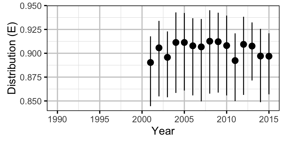
Abundance - Mountain Whitefish - Adult

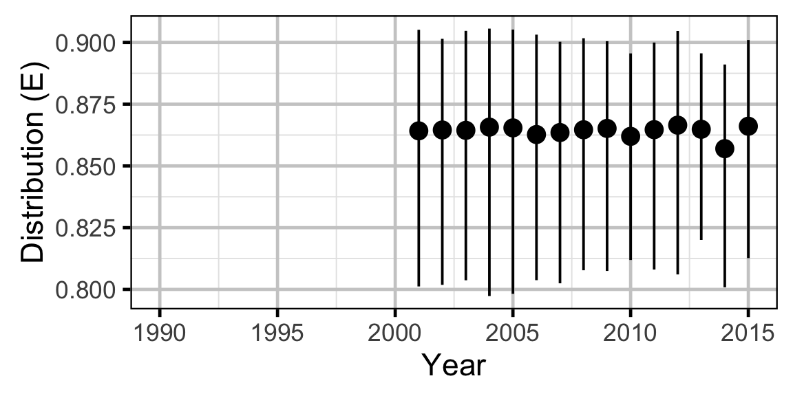
Abundance - Rainbow Trout - Subadult

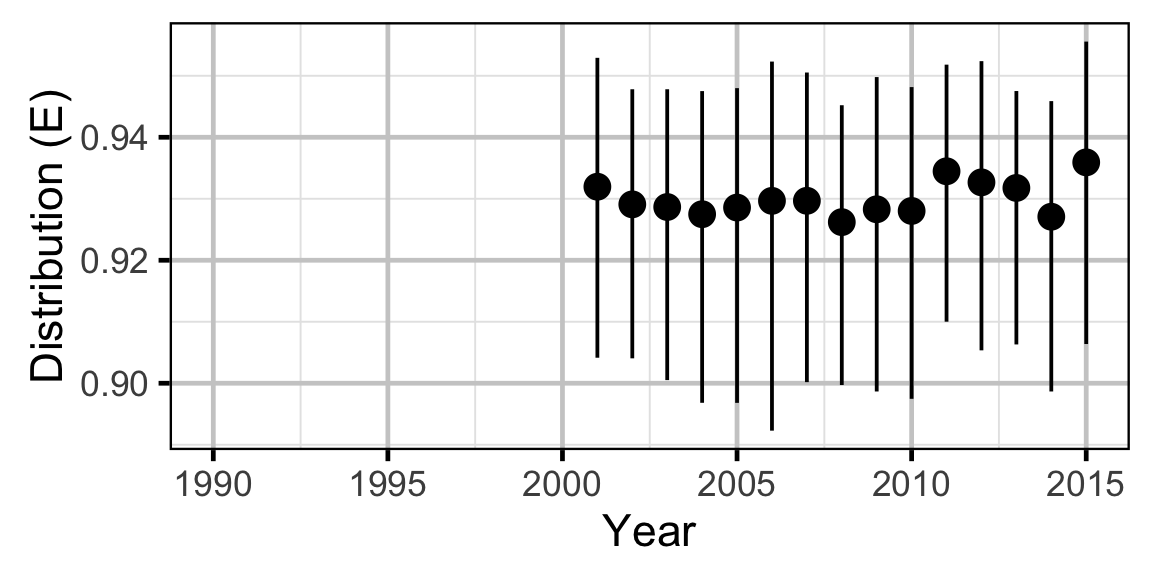
Abundance - Rainbow Trout - Adult

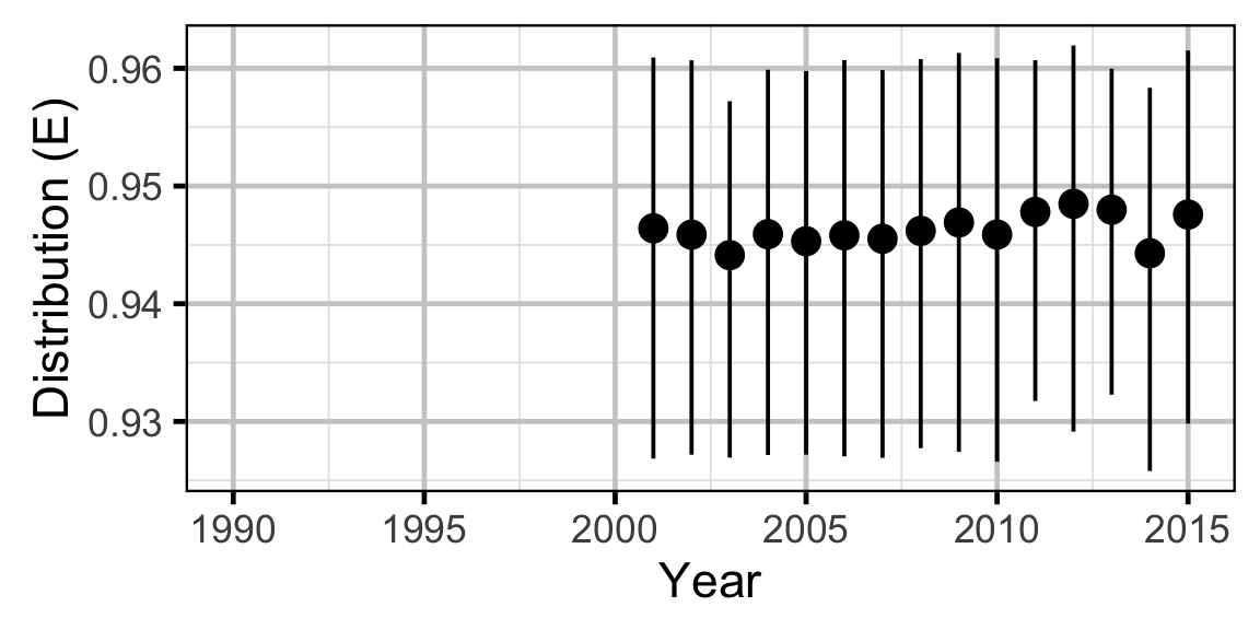
Abundance - Walleye - Adult

Long-Term Trends

Short-Term Correlations
Scale Age
Age-Ratios
Stock-Recruitment - Mountain Whitefish
Stock-Recruitment - Rainbow Trout
Acknowledgements
The organisations and individuals whose contributions have made this analysis report possible include:
- BC Hydro
- Okanagan Nation Alliance
- Amy Duncan
- Golder Associates
- Demitria Burgoon
- Dustin Ford
- David Roscoe
- Sima Usvyatsov
- Dana Schmidt
- Larry Hildebrand
References
Abmann, C., J. Boysen-Hogrefe, and M. Pape. 2014. “Bayesian Analysis of Dynamic Factor Models: An Ex-Post Approach Towards the Rotation Problem.” Kiel Working Paper No. 1902. Kiel, Germany: Kiel Institute for the World Economy.
Bradford, Michael J, Josh Korman, and Paul S Higgins. 2005. “Using Confidence Intervals to Estimate the Response of Salmon Populations (Oncorhynchus Spp.) to Experimental Habitat Alterations.” Canadian Journal of Fisheries and Aquatic Sciences 62 (12): 2716–26. https://doi.org/10.1139/f05-179.
Fabens, A J. 1965. “Properties and Fitting of the von Bertalanffy Growth Curve.” Growth 29 (3): 265–89.
He, Ji X., James R. Bence, James E. Johnson, David F. Clapp, and Mark P. Ebener. 2008. “Modeling Variation in Mass-Length Relations and Condition Indices of Lake Trout and Chinook Salmon in Lake Huron: A Hierarchical Bayesian Approach.” Transactions of the American Fisheries Society 137 (3): 801–17. https://doi.org/10.1577/T07-012.1.
Hurlbert, S. 1984. “Pseudoreplication and the Design of Ecological Field Experiments.” Ecological Monographs 54 (2): 187–211.
Irvine, R. L., J. T. A. Baxter, and J. L. Thorley. 2015. “Lower Columbia River Rainbow Trout Spawning Assessment: Year 7 (2014 Study Period).” A Mountain Water Research and Poisson Consulting Ltd. Report. Castlegar, B.C.: BC Hydro. http://www.bchydro.com/content/dam/BCHydro/customer-portal/documents/corporate/environment-sustainability/water-use-planning/southern-interior/clbmon-46-yr7-2015-02-04.pdf.
Kery, Marc. 2010. Introduction to WinBUGS for Ecologists: A Bayesian Approach to Regression, ANOVA, Mixed Models and Related Analyses. Amsterdam; Boston: Elsevier. http://public.eblib.com/EBLPublic/PublicView.do?ptiID=629953.
Kery, Marc, and Michael Schaub. 2011. Bayesian Population Analysis Using WinBUGS : A Hierarchical Perspective. Boston: Academic Press. http://www.vogelwarte.ch/bpa.html.
Macdonald, P. D. M., and T. J. Pitcher. 1979. “Age-Groups from Size-Frequency Data: A Versatile and Efficient Method of Analyzing Distribution Mixtures.” Journal of the Fisheries Research Board of Canada 36 (8): 987–1001. https://doi.org/10.1139/f79-137.
Plummer, Martyn. 2015. “JAGS Version 4.0.1 User Manual.” http://sourceforge.net/projects/mcmc-jags/files/Manuals/4.x/.
R Core Team. 2015. “R: A Language and Environment for Statistical Computing.” Vienna, Austria: R Foundation for Statistical Computing. http://www.R-project.org/.
Subbey, S., J. A. Devine, U. Schaarschmidt, and R. D. M. Nash. 2014. “Modelling and Forecasting Stock-Recruitment: Current and Future Perspectives.” ICES Journal of Marine Science 71 (8): 2307–22. https://doi.org/10.1093/icesjms/fsu148.
Thorley, J. L. 2013. “Jaggernaut: An R Package to Facilitate Bayesian Analyses Using JAGS (Just Another Gibbs Sampler).” Nelson, B.C.: Poisson Consulting Ltd. https://github.com/poissonconsulting/jaggernaut.
Tornqvist, Leo, Pentti Vartia, and Yrjo O. Vartia. 1985. “How Should Relative Changes Be Measured?” The American Statistician 39 (1): 43. https://doi.org/10.2307/2683905.
von Bertalanffy, L. 1938. “A Quantitative Theory of Organic Growth (Inquiries on Growth Laws Ii).” Human Biology 10: 181–213.
Walters, Carl J., and Steven J. D. Martell. 2004. Fisheries Ecology and Management. Princeton, N.J: Princeton University Press.
Zuur, A F, I D Tuck, and N Bailey. 2003. “Dynamic Factor Analysis to Estimate Common Trends in Fisheries Time Series.” Canadian Journal of Fisheries and Aquatic Sciences 60 (5): 542–52. https://doi.org/10.1139/f03-030.