Lower Columbia River Fish Population Indexing Analysis 2013

The suggested citation for this analytic report is:

Thorley, J.L. (2014) Lower Columbia River Fish Population Indexing Analysis 2013. A Poisson Consulting Analysis Report. URL: https://www.poissonconsulting.ca/f/252359126.

Background

In the mid 1990s BC Hydro began operating Hugh L. Keenleyside (HLK) Dam to reduce dewatering of Mountain Whitefish and Rainbow Trout eggs.

The primary goal of the Lower Columbia River Fish Population Indexing program is to answer two key management questions:

What are the abundance, growth rate, survival rate, body condition, age distribution, and spatial distribution of subadult and adult Whitefish, Rainbow Trout, and Walleye in the LCR?

What is the effect of inter-annual variability in the Whitefish and Rainbow Trout flow regimes on the abundance, growth rate, survival rate, body condition, and spatial distribution of subadult and adult Whitefish, Rainbow Trout, and Walleye in the LCR?

Methods

Data Preparation

The fish indexing data were provided by Golder Associates in the form of an Access database. The discharge and temperature data were queried from a BC Hydro database maintained by Poisson Consulting.

The data were prepared for analysis using R version 3.1.0 (Team (2013)).

Statistical Analysis

Hierarchical Bayesian models were fitted to the fish indexing data data using R version 3.1.0 (Team (2013)) and JAGS 3.4.0 (Plummer (2012)) which interfaced with each other via jaggernaut 1.8.2 (Thorley (2014)). For additional information on hierarchical Bayesian modelling in the BUGS language, of which JAGS uses a dialect, the reader is referred to Kery and Schaub (2011) pages 41-44.

Unless specified, the models assumed vague (low information) prior distributions (Kéry and Schaub (2011)36). The posterior distributions were estimated from a minimum of 1,000 Markov Chain Monte Carlo (MCMC) samples thinned from the second halves of three chains (Kéry and Schaub (2011)38-40). Model convergence was confirmed by ensuring that Rhat (Kéry and Schaub (2011)40) was less than 1.1 for each of the parameters in the model (Kéry and Schaub (2011)61). Model adequacy was confirmed by examination of residual plots.

The posterior distributions of the fixed (Kéry and Schaub (2011)75) parameters are summarised in terms of a point estimate (mean), lower and upper 95% credible limits (2.5th and 97.5th percentiles), the standard deviation (SD), percent relative error (half the 95% credible interval as a percent of the point estimate) and significance (Kéry and Schaub (2011)37,42).

Variable selection was achieved by dropping uninformative explanatory variables where a variable was considered to be uninformative if its percent relative error was \(\geq\) 100%. In the case of fixed effects this is approximately equivalent to dropping insignificant variables, i.e., those with a significance \(\geq\) 0.05.

The results are displayed graphically by plotting the modeled relationships between particular variables and the response with 95% credible intervals (CRIs) with the remaining variables held constant. In general, continuous and discrete fixed variables are held constant at their mean and first level values respectively while random variables are held constant at their typical values (expected values of the underlying hyperdistributions) (Kéry and Schaub (2011)77-82). Where informative the influence of particular variables is expressed in terms of the effect size (i.e., percent change in the response variable) with 95% CRIs (Bradford et al. (2005)). Plots were produced using the ggplot2 R package (Wickham (2009)).

Condition

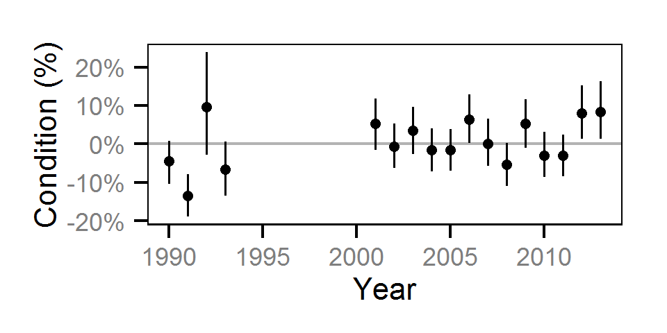
Condition was estimated via an analysis of weight-length relations (He et al. (2008)).

Key assumptions of the condition model include:

  • Weight varies with length and date.
  • Weight varies randomly with year.
  • The relationship between length and weight varies with date.
  • The relationship between length and weight varies randomly with year.
  • The effect of year on weight is correlated with the effect of year on the relationship between length and weight.
  • The residual weight variation in weight is log-normally distributed.

Only previously untagged fish were included in models to avoid potential effects of tagging on body condition.

Growth

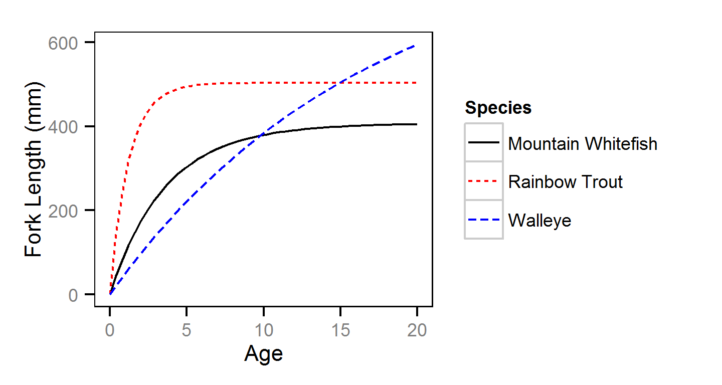
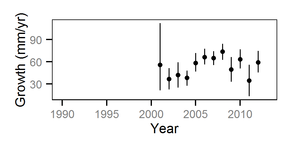
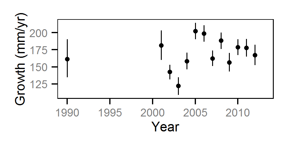
Annual growth was estimated from the inter-annual recaptures using the Fabens method (Fabens (1965)) for estimating the von Bertalanffy growth curve (Bertalanffy (1938)).

Key assumptions of the growth model include:

  • The growth coefficient (k) varies randomly with year.
  • The residual growth variation is normally distributed.

Length-At-Age

The length-at-age of Mountain Whitefish and Rainbow Trout was estimated from the annual length-frequency distributions using a finite mixture distribution model (MacDonald and Pitcher 1979).

Key assumptions of the length-at-age model include:

  • There are three distinguishable age-classes for each species: age-0, age-1 and age-2 and older. - Length increases with age-class.
  • Length varies as a second-order polynomial of date;
  • Length varies randomly by year within age-class.
  • The proportion of individuals belonging to each age-class remained constant among years.
  • Individual variation in length is normally distributed.

The model was used to estimate the cut-offs between age-0, age-1 and age-2 and older individuals by year. For the purposes of estimating other population parameters by life stage, age-0 individuals were classified as fry, age-1 individuals were classified as subadult, and age-2 and older individuals were classified as adult. Walleye could not be separated by life stage due to a lack of discrete modes in the length-frequency distributions for this species. Consequently, all captured Walleye were considered to be adults.

Length Bias

The bias in observer’s fish length estimates was quantified using a model with a categorical distribution that compared the proportions of fish in different length-classes for each observer in 2013 to the equivalent proportions for the measured fish.

Key assumptions of the length bias model include:

  • The percent bias varies by observer.
  • The percent bias is constant by fish length.

The observer’s fish lengths were corrected for the estimated bias before being classified as fry, subadult and adult based on the length-at-age cutoffs.

Survival

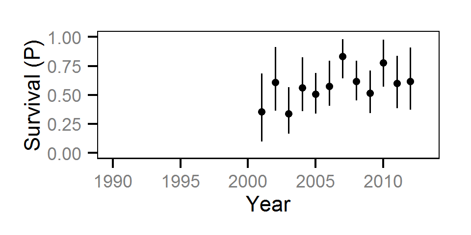
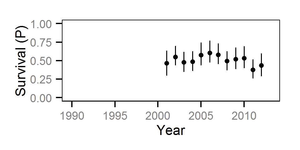
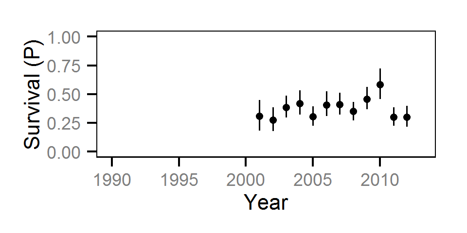
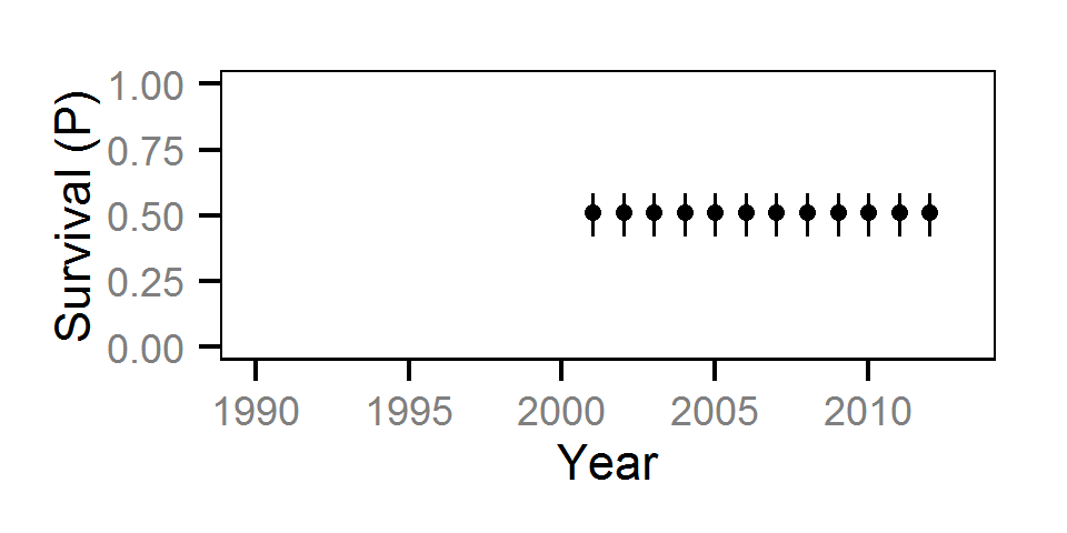
The annual survival rate was estimated by fitting a Cormack-Jolly-Seber model (Kéry and Schaub (2011)172-177) to inter-annual recaptures.

Key assumptions of the survival model include:

  • Survival varies randomly with year within life stage.
  • The encounter probability is constant across years.

Site Fidelity

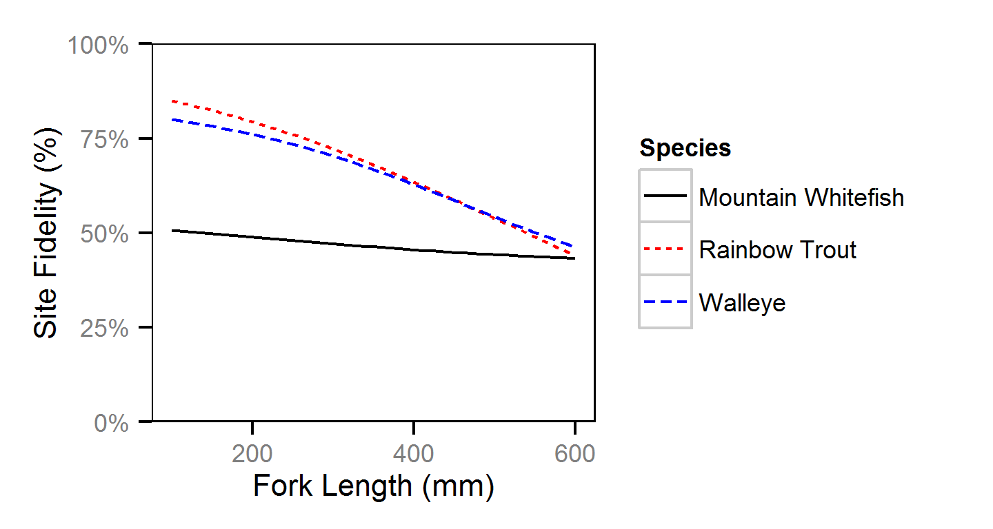
The probability of a recaptured fish being caught at the same site at which it was previously encountered versus a different site (the site fidelity) was estimated using a logistic regression.

Key assumptions of the site fidelity model include:

  • The site fidelity varies with body length.

Capture Efficiency

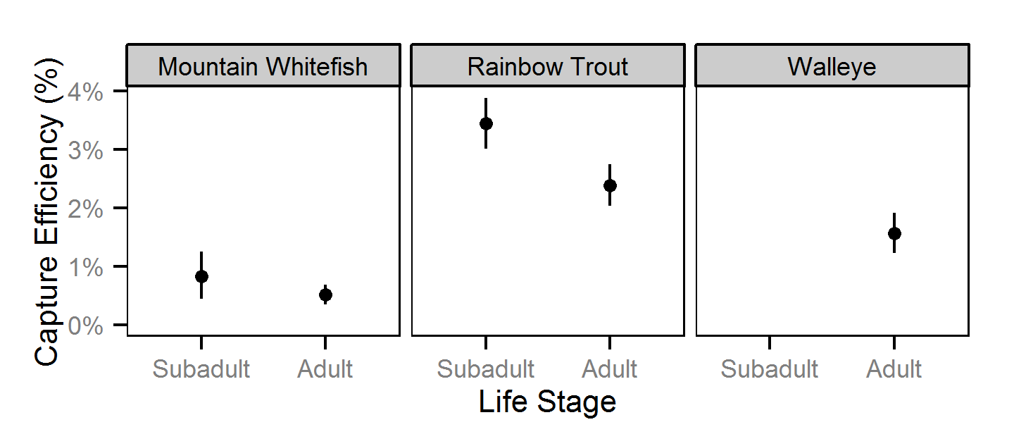
The probability of capture was estimated using a recapture-based binomial model (Kéry and Schaub (2011)134-136, 384-388).

Key assumptions of the capture efficiency model include:

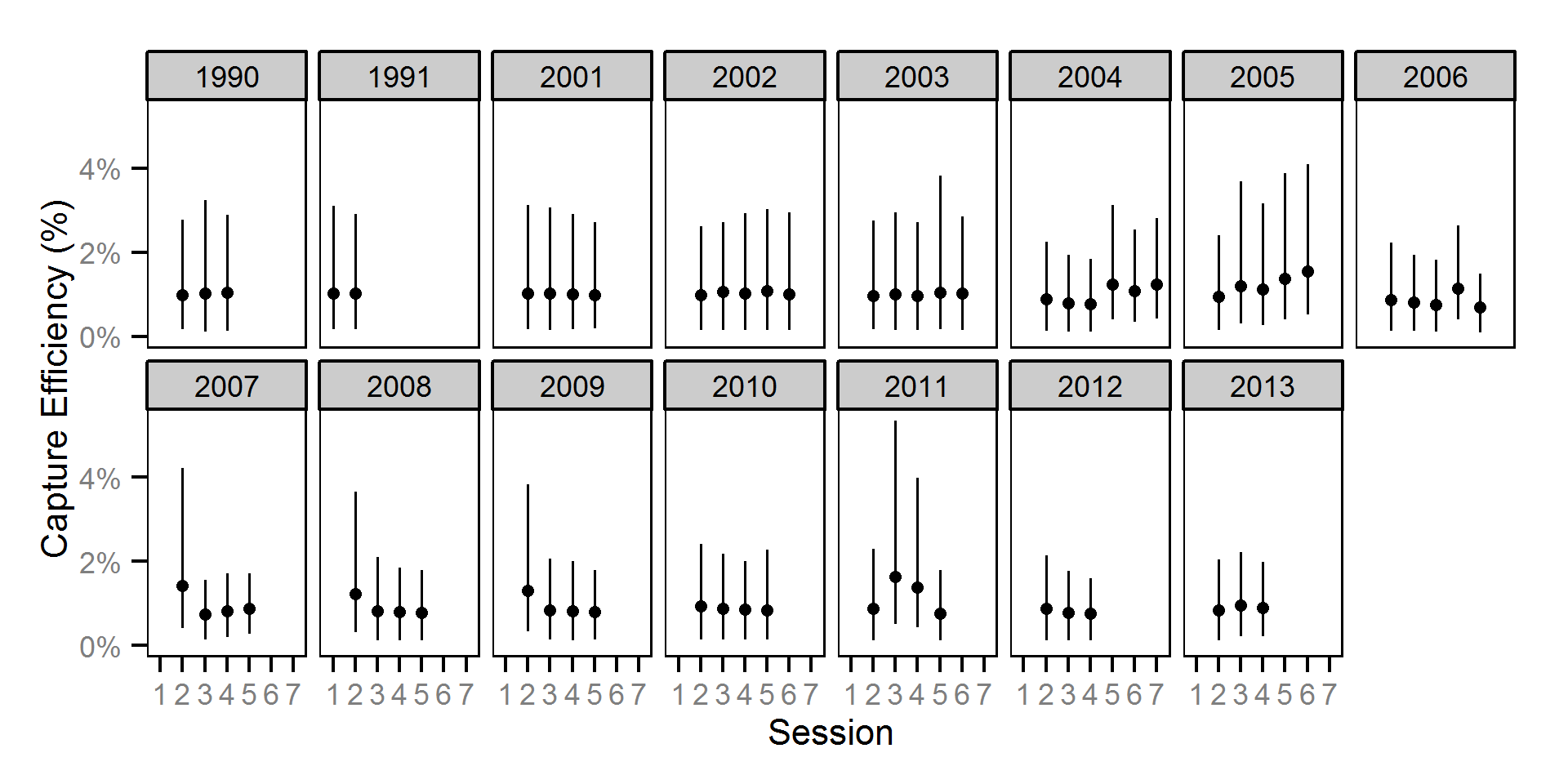
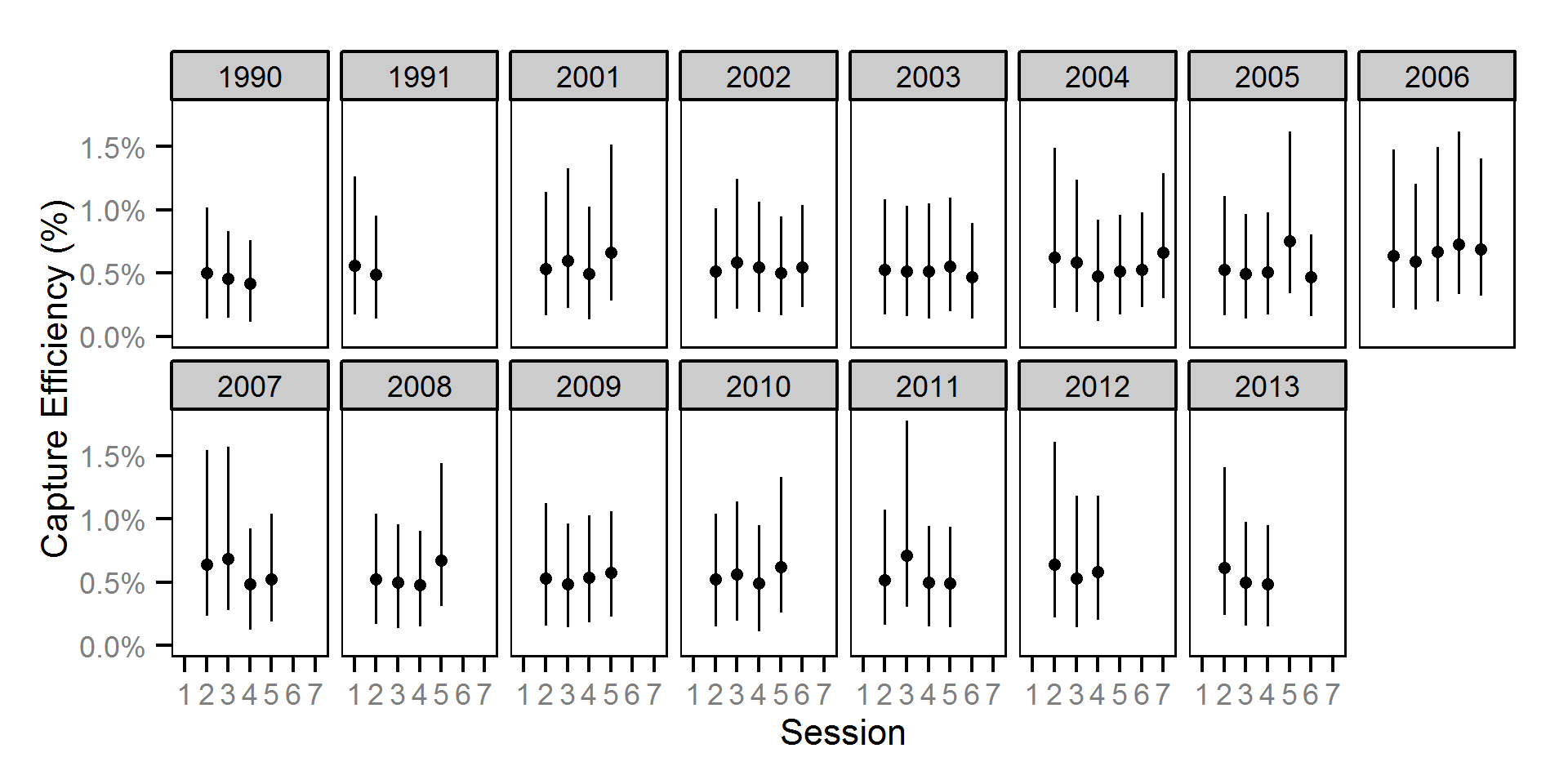
  • The capture probability varies randomly by session within year.
  • The probability of a marked fish remaining at a site is the estimated site fidelity.
  • The number of recaptures is described by a binomial distribution.

Abundance

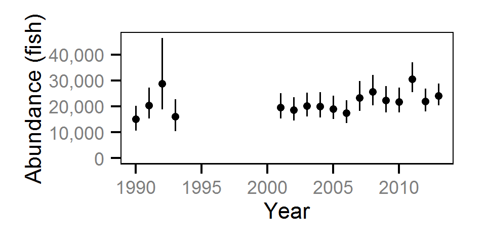
The abundance was estimated from the catch and bias-corrected observer count data using an overdispersed Poisson model (Kéry and Schaub (2011)55-56). The model assumed that the capture efficiency was the mean estimate from the capture efficiency model and that the number of observed fish was a multiple of the number of captured fish. The annual abundance estimates represent the total number of fish in the study area.

Key assumptions of the abundance model include:

  • The capture efficiency is the mean estimate from the capture efficiency model.
  • The observer efficiency varies from the capture efficiency.
  • The lineal fish density varies randomly with site, year and site within year.
  • The catches and counts are described by a Poisson-gamma distribution.

Dynamic Factor Analysis

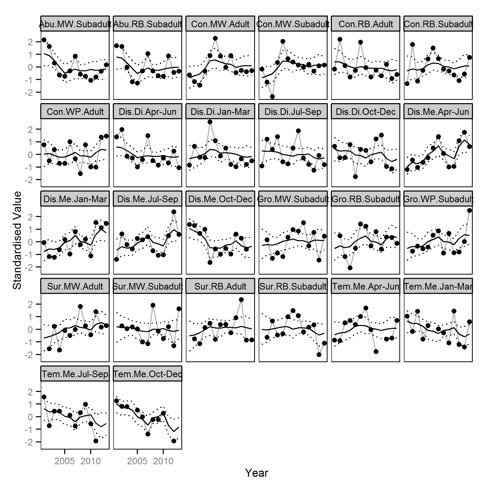
Trends common to the fish index and environmental annual time series were identified using Dynamic Factor Analysis (Zuur et al. (2003)) - a dimension-reduction technique especially designed for time-series data.

The fish index time series were the growth (Gro..), condition (Con..), survival (Sur..) and abundance (Abu..) by species code and life stage. The annual abundance of adults were excluded as the values are the result of survival and subadult abundance across multiple years.

The environmental time series were the mean discharge (Dis.Me..), and the average hourly absolute discharge difference (Dis.Di..) at Birchbank and the average water temperature (Tem.Me..) at Norns Creek by quaterly period. The average hourly absolute discharge difference was calculated by differencing the mean hourly discharge time series and taking the average of the absolute differences. Mathematically this is equivalent to

\[ \frac{\sum |x_{1}-x_{2}| + |x_{2}-x_{3}| + ... + |x_{n-1}-x_{n}|}{n-1} \] where \(x_{1}\) is the discharge at the start of the time series and \(x_{2}\) is the discharge an hour later.

The ..Oct-Dec times series were lead (opposite of lagged) by one year as they were not expected to influence the fish time series in the same year.

All time series were standardized prior to fitting the DFA model. Key assumptions of the dynamic factor analysis model include:

  • The trends are described by independent random walks with a shared standard deviation.
  • The expected value is the sum of the time series weighted trends.
  • The SD of the residual variation varies by time series.
  • The residual variation is normally distributed.

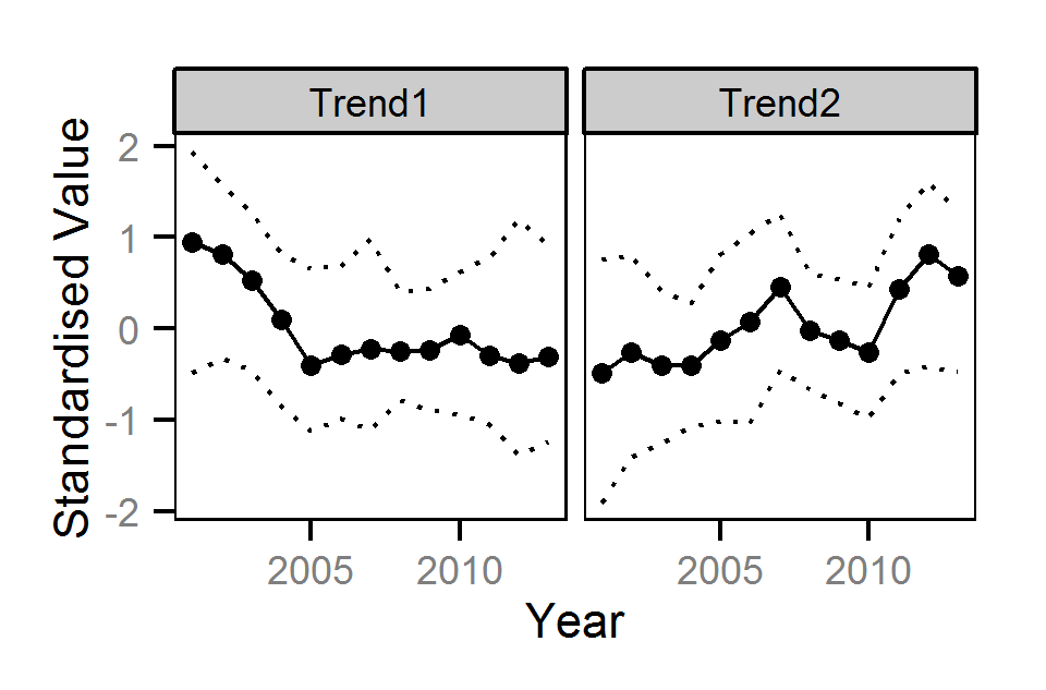
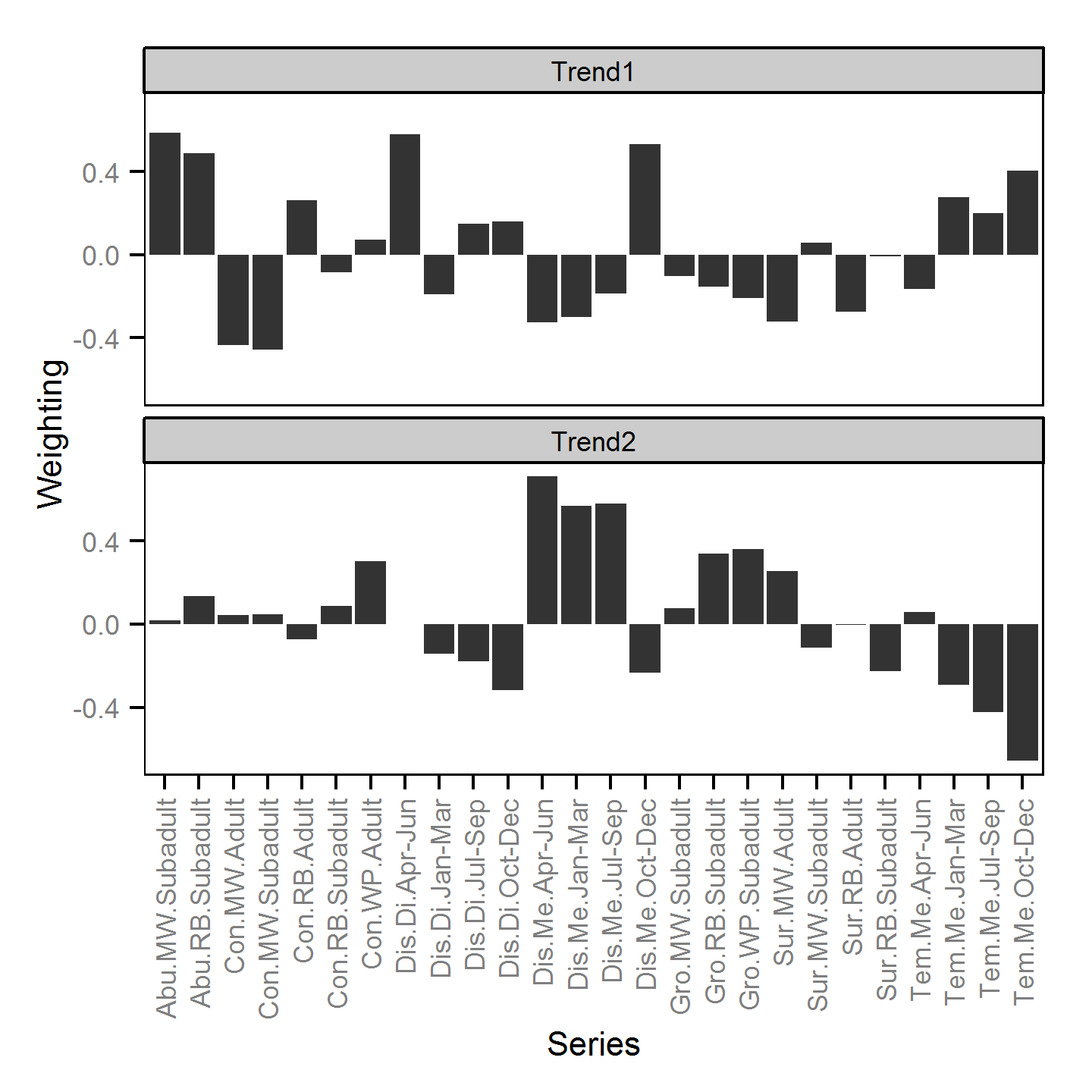
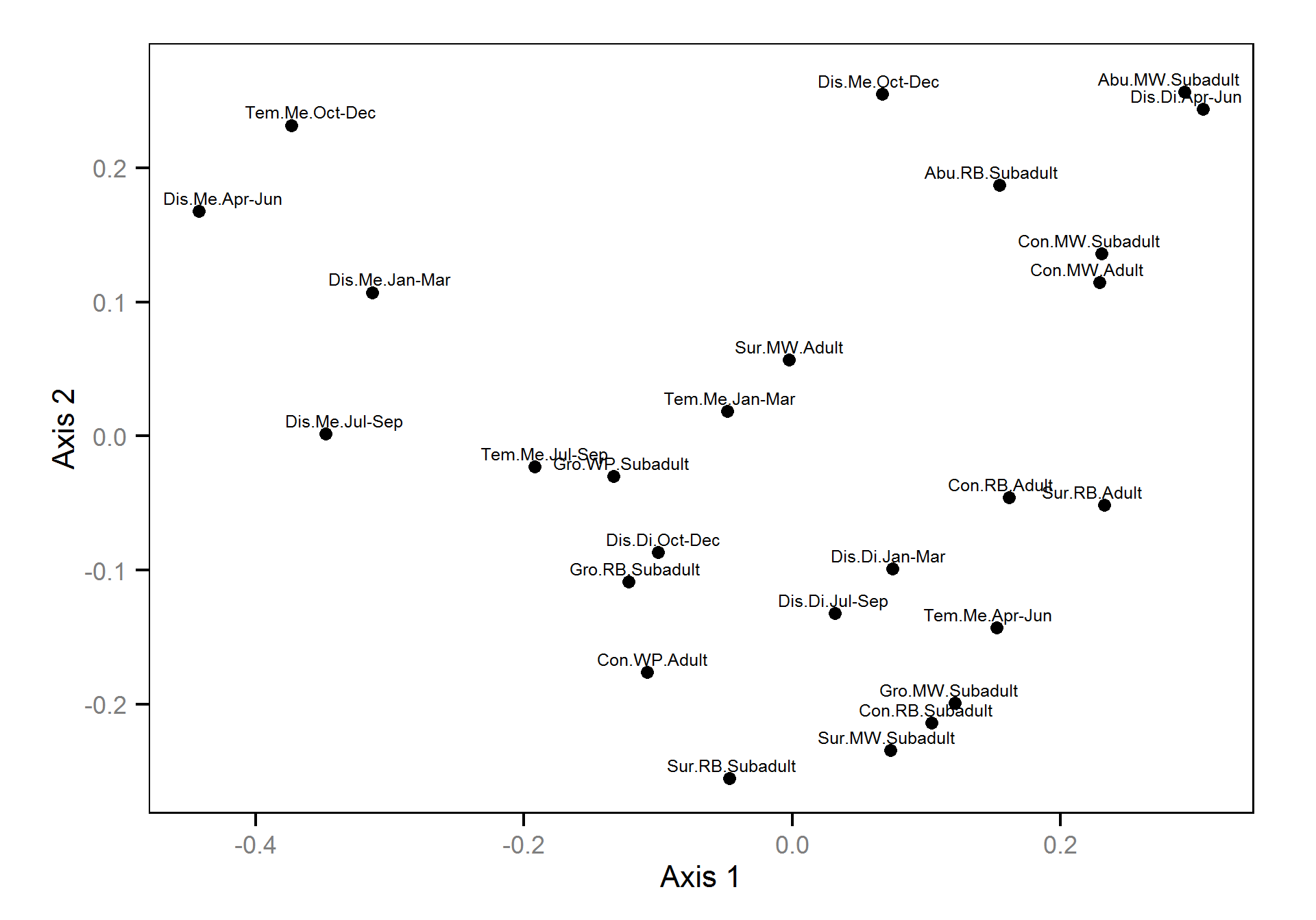
Preliminary analyses indicated that two trends provided a reasonable model fit without apparent over-fitting. Non-metric multidimensional scaling was used to indicate the clustering of time series based on the absolute DFA trend weightings

Model Code

The JAGS model code, which uses a series of naming conventions, is presented below.

Condition

Variable/Parameter Description
bCorrelation Correlation coefficient between sWeightYear and sWeightLengthYear
bWeight Intercept for eLogWeight
bWeightDayte Effect of Dayte on eLogWeight
bWeightLength Effect of Length on eLogWeight
bWeightLengthDayte Effect of Dayte on effect of Length on eLogWeight
bWeightLengthYear Effect of Year on effect of Length on eLogWeight
bWeightYear Effect of Year on eLogWeight
Dayte[i] Day of year ith fish was captured
eLogWeight[i] Expected log(weight) of ith fish
Length[i] Log length of ith fish
sWeight SD of residual variation in log(Weight)
sWeightLengthYear SD of effect of Year on effect of Length on eLogWeight
sWeightYear SD of effect of Year on eLogWeight
Weight[i] Observed weight of ith fish
Year[i] Year ith fish was captured
Condition - Model1
model {

  bWeight ~ dnorm(5, 5^-2)
  bWeightLength ~ dnorm(3, 5^-2)

  bWeightDayte ~ dnorm(0, 5^-2)
  bWeightLengthDayte ~ dnorm(0, 5^-2)

  eMu[1] <- bWeight
  eMu[2] <- bWeightLength

  dR[1,1] <- 0.1
  dR[1,2] <- 0
  dR[2,1] <- 0
  dR[2,2] <- 0.1

  eOmega ~ dwish(dR, 2)

  for (i in 1:nYear) {
  eYear[i, 1:2] ~ dmnorm(eMu, eOmega)
  bWeightYear[i] <- eYear[i, 1] - bWeight
  bWeightLengthYear[i] <- eYear[i, 2] - bWeightLength
  }

  eS2 <-inverse(eOmega)
  sWeightYear <- sqrt(eS2[1,1])
  sWeightLengthYear <- sqrt(eS2[2,2])
  bCorrelation <- eS2[1,2] / sqrt(eS2[1,1] * eS2[2,2]) 

  sWeight ~ dunif(0, 5)
  for(i in 1:length(Length)) {

  eLogWeight[i] <- bWeight + bWeightDayte * Dayte[i] +  bWeightYear[Year[i]] + (bWeightLength + bWeightLengthDayte * Dayte[i] + bWeightLengthYear[Year[i]]) * Length[i]

  Weight[i] ~ dlnorm(eLogWeight[i], sWeight^-2)
  }
  }

Growth

Variable/Parameter Description
bK Intercept for log(eK)
bKYear[i] Effect of ith year on log(eK)
bLinf Mean maximum length
eGrowth[i] Expected growth between release and recapture of ith recapture
eK[i] Expected von Bertalanffy growth coefficient in ith year
Growth[i] Observed growth between release and recapture of ith recapture
LengthAtRelease[i] Previous length at release of ith recapture
sGrowth SD of residual variation in Growth
sKYear SD of effect of ith year on log(eK)
Year[i] Release year of ith recapture
Years[i] Years between release and recapture of ith recapture
Growth - Model1
model {

  bK ~ dnorm (0, 5^-2)

  sKYear ~ dunif (0, 5)
  for (i in 1:nYear) {
    bKYear[i] ~ dnorm(0, sKYear^-2)
    log(eK[i]) <- bK + bKYear[i]
  }

  bLinf ~ dunif(100, 1000)
  sGrowth ~ dunif(0, 100)

  for (i in 1:length(Year)) {
    eGrowth[i] <- (bLinf - LengthAtRelease[i]) * (1 - exp(-sum(eK[Year[i]:(Year[i] + Years[i] - 1)])))

    Growth[i] ~ dnorm(eGrowth[i], sGrowth^-2)
  }
}

Length-At-Age

Variable/Parameter Description
Age[i] Age of ith fish observed
bAgeYear Effect of Age within Year on eLength
bDayte[j] Linear effect of Dayte on eLength for a jth aged fish
bDayte2[j] Quadratic effect of Dayte on eLength for a jth aged fish
bIntercept[j] Intercept of eLength for a jth aged fish
Dayte[i] Day of year ith fish was observed
eIncrement[i] Length difference between an ith aged fish and an (i-1)th aged fish
eLength[i] Expected length of ith fish
Length[i] Observed length of ith fish
pAge[i] Proportion of fish belonging to jth age
sAgeYear SD of effect of Age within Year on eLength
sLengthAge[j] SD of residual variation in eLength for a jth aged fish
Year[i] Year ith fish was observed
Length-At-Age - Model1

model {
  for(i in 1:nAge)  {
    dAge[i] <- 1

    eIncrement[i] ~ dunif(50, 250)

    bDayte[i] ~ dnorm(0, 10)
    bDayte2[i] ~ dnorm(0, 10)

    sAgeYear[i] ~ dunif(0, 50)
    for(j in 1:nYear) {
      bAgeYear[i, j] ~ dnorm(0, sAgeYear[i]^-2)     }
    sLengthAge[i] ~ dunif(0, 100)
  }

  bIntercept[1] <- eIncrement[1]
  for(i in 2:nAge) {
    bIntercept[i] <- bIntercept[i-1] + eIncrement[i]
  }

  pAge[1:nAge] ~ ddirch(dAge[]) 

  for (i in 1:length(Length)) {
    Age[i] ~ dcat(pAge[])
    eLength[i] <- bIntercept[Age[i]] + bDayte[Age[i]] * Dayte[i] + bDayte2[Age[i]] * Dayte[i]^2 + bAgeYear[Age[i],Year[i]]
    Length[i] ~ dnorm(eLength[i], sLengthAge[Age[i]]^-2)
  }
}

Length Bias

Variable/Parameter Description
bLength Effect of Observer on eLength
ClassWidth Width of classes
eLength[i] Expected actual length class of ith fish
Length[i] Observed length of ith fish
Observer[i] Observer of ith fish
sLength SD of residual variation in length class
Length Bias - Model1
model {
  for(i in 1:Classes) {
    dLengthClass[i] <- 1
  }

  pLengthClass[1:Classes] ~ ddirch(dLengthClass[])

  bLength[1] <- 1
  sLength[1] <- 0.01
  for(i in 2:nObserver) {
    bLength[i] ~ dunif(0.5, 2)
    sLength[i] ~ dunif(0.5, 2)
  }

  for(i in 1:length(Length))  {
    eLengthClass[i] ~ dcat(pLengthClass[])
    eLength[i] <- bLength[Observer[i]] * eLengthClass[i] 
    Length[i] ~ dnorm(eLength[i] * ClassWidth, (sLength[Observer[i]] * ClassWidth)^-2)
  }
}

Survival

Variable/Parameter Description
bEfficiency Intercept for logit(eEfficiency)
bSurvivalInterceptStage Intercept for logit(eSurvival) by Stage
bSurvivalStageYear Effect of Year on logit(eSurvival) by Stage
eAlive[i, j] Expected state (alive or dead) of ith fish in jth year
eEfficiency[i, j] Expected recapture probability of ith fish in jth year
eSurvival[i, j] Expected survival probability of ith fish in jth year
FirstYear[i] First year ith fish was observed
FishYear[i, j] Whether ith fish was observed in jth year
sSurvivalStageYear SD of effect of Year on logit(eSurvival) by Stage
StageFishYear[i, j] Stage of ith fish in jth year
Survival - Model1
model {

  bEfficiency ~ dnorm (0, 5^-2)

  for (i in 1:nStage) {
    sSurvivalStageYear[i] ~ dunif (0, 5)
  }

  for(i in 1:nStage) {
    bSurvivalInterceptStage[i] ~ dnorm(0, 5^-2)
    for (j in 1:nYear) {
      bSurvivalStageYear[i,j] ~ dnorm (0, sSurvivalStageYear[i]^-2)
    }
  }

  for (i in 1:nFish) {
    eAlive[i, FirstYear[i]] <- 1
    for (j in (FirstYear[i]+1):nYear) {
      logit(eEfficiency[i,j]) <- bEfficiency

      logit(eSurvival[i,j-1]) <- bSurvivalInterceptStage[StageFishYear[i,j-1]] + bSurvivalStageYear[StageFishYear[i,j-1],j-1]
      eAlive[i,j] ~ dbern (eAlive[i,j-1] * eSurvival[i,j-1])
      FishYear[i,j] ~ dbern (eAlive[i,j] * eEfficiency[i,j])
    }
  }
}

Site Fidelity

Variable/Parameter Description
bFidelity Intercept for logit(eFidelity)
bLength Effect of Length on logit(eFidelity)
eFidelity[i] Expected site fidelity for ith recapture
Fidelity[i] Whether or not ith recapture was encounterd at the same site as the previous encounter
Length[i] Length of ith recapture at previous encounter
Site Fidelity - Model1
model {
  bFidelity ~ dnorm(0, 2^-2)
  bLength ~ dnorm(0, 2^-2)

  for (i in 1:length(Fidelity)) {
    logit(eFidelity[i]) <- bFidelity + bLength * Length[i] 
    Fidelity[i] ~ dbern(eFidelity[i])
  }
}

Capture Efficiency

Variable/Parameter Description
bEfficiency Intercept for logit(eEfficiency)
bEfficiencySessionYear Effect of Session within Year on logit(eEfficiency)
eEfficiency[i] Expected efficiency on ith visit
eFidelity[i] Expected site fidelity on ith visit
Fidelity[i] Mean site fidelity on ith visit
FidelitySD[i] SD of site fidelity on ith visit
Recaptures[i] Number of marked fish recaught during ith visit
sEfficiencySessionYear SD of effect of Session within Year on logit(eEfficiency)
Session[i] Session of ith visit
Tagged[i] Number of marked fish tagged prior to ith visit
Year[i] Year of ith visit
Capture Efficiency - Model1
model {

  bEfficiency ~ dnorm(0, 5^-2)

  sEfficiencySessionYear ~ dunif(0, 2)
  for (i in 1:nSession) {
    for (j in 1:nYear) {
      bEfficiencySessionYear[i, j] ~ dnorm(0, sEfficiencySessionYear^-2)
    }
  }

  for(i in 1:length(Year)) {
    logit(eEfficiency[i]) <- bEfficiency + bEfficiencySessionYear[Session[i], Year[i]]
    eFidelity[i] ~ dnorm(Fidelity[1], FidelitySD[1]^-2) T(0, 1)
    Recaptures[i] ~ dbin(eEfficiency[i] * eFidelity[i], Tagged[i])
  }
}

Abundance

Variable/Parameter Description
bDensity Intercept for log(eDensity)
bDensitySite Effect of Site on log(eDensity)
bDensitySiteYear Effect of Site within Year on log(eDensity)
bDensityYear Effect of Year on log(eDensity)
bType Effect of Type on Efficiency
Count[i] Observed count during ith visit
eDensity[i] Expected density during ith visit
eDispersion Overdispersion of Count
Efficiency[i] Survey efficiency during ith visit
ProportionSampled[i] Proportion of site surveyed during ith visit
sDensitySite SD of effect of Site on log(eDensity)
sDensitySiteYear SD of effect of Site within Year on log(eDensity)
sDensityYear SD of effect of Year on log(eDensity)
sDispersion SD of overdispersion term
Site[i] Site of ith visit
SiteLength[i] Length of site during ith visit
Type[i] Survey type (catch versus count) during ith visit
Year[i] Year of ith visit
Abundance - Model1
model {

  bDensity ~ dnorm(5, 5^-2)

  bType[1] <- 1
  for (i in 2:nType) {
    bType[i] ~ dunif(0, 10)
  }

  sDensityYear ~ dunif(0, 2)
  for (i in 1:nYear) {
    bDensityYear[i] ~ dnorm(0, sDensityYear^-2)
  }

  sDensitySite ~ dunif(0, 2)
  sDensitySiteYear ~ dunif(0, 2)
  for (i in 1:nSite) {
    bDensitySite[i] ~ dnorm(0, sDensitySite^-2)
    for (j in 1:nYear) {
      bDensitySiteYear[i, j] ~ dnorm(0, sDensitySiteYear^-2)
    }
  }

  sDispersion ~ dunif(0, 5)
  for (i in 1:length(Count)) {
    log(eDensity[i]) <- bDensity + bDensitySite[Site[i]] + bDensityYear[Year[i]] + bDensitySiteYear[Site[i],Year[i]]

    eDispersion[i] ~ dgamma(1 / sDispersion^2, 1 / sDispersion^2)    
    Count[i] ~ dpois(eDensity[i] * SiteLength[i] * ProportionSampled[i] * Efficiency[i] * bType[Type[i]] * eDispersion[i])  
  }
}

Dynamic Factor Analysis

Variable/Parameter Description
bTrend[i,j] Value of ith trend in jth Year
bWeighting[i,j] Weighting of ith Trend for jth Series
Series[i] Time series of ith value
sSeries[i] SD for ith Series
sTrend SD for bTrend
Value[i] ith value
Year[i] Year of ith value
Dynamic Factor Analysis - Model1
model {

  sTrend ~ dunif(0, 1)
  for(i in 1:nTrend) {
    muTrend[i] <- 0
    for(j in 1:nTrend) {
      oTrend[i,j] <- ifelse(i == j, sTrend^-2, 0)
    }
    for(j in 1:nSeries) {
      eWeighting[i,j] ~ dunif(-1, 1)
      aWeighting[i,j] <- eWeighting[i,j] * ifelse(j < nTrend andand i > j, 0, 1)
      bWeighting[i,j] <- ifelse(j <= nTrend andand i == j, abs(aWeighting[i,j]), aWeighting[i,j])
    }
  }
  bTrend[1:nTrend, 1] ~ dmnorm(muTrend, oTrend / 25)
  for(j in 2:nYear) {
    bTrend[1:nTrend, j] ~ dmnorm(bTrend[1:nTrend,j-1], oTrend)
  }

  for(i in 1:nSeries) {
    sSeries[i] ~ dunif(0, 1)
  }

  for(i in 1:length(Value)) {
    eValue[i] <- sum(bWeighting[,Series[i]] * bTrend[,Year[i]])
    Value[i] ~ dnorm(eValue[i], sSeries[Series[i]]^-2)
  }
}
Results

Model Parameters

The posterior distributions for the fixed (Kery and Schaub 2011 p. 75) parameters in each model are summarised below.

Condition - Mountain Whitefish

Parameter Estimate Lower Upper SD Error Significance
bCorrelation 0.3070 -0.1679 0.6668 0.2194 136 0.1816
bWeight 5.5472 5.5027 5.5943 0.0231 1 0.0000
bWeightDayte -0.0118 -0.0156 -0.0079 0.0020 33 0.0000
bWeightLength 3.1346 3.0384 3.2246 0.0449 3 0.0000
bWeightLengthDayte -0.0062 -0.0169 0.0044 0.0055 172 0.2415
sWeight 0.1580 0.1564 0.1596 0.0009 1 0.0000
sWeightLengthYear 0.1827 0.1277 0.2658 0.0355 38 0.0000
sWeightYear 0.0936 0.0686 0.1330 0.0164 34 0.0000
Rhat Iterations
1.02 10000

Condition - Rainbow Trout

Parameter Estimate Lower Upper SD Error Significance
bCorrelation 0.0605 -0.4120 0.5025 0.2360 756 0.8004
bWeight 5.8789 5.8388 5.9224 0.0216 1 0.0000
bWeightDayte -0.0051 -0.0078 -0.0025 0.0014 52 0.0000
bWeightLength 2.9229 2.8737 2.9705 0.0249 2 0.0000
bWeightLengthDayte 0.0457 0.0381 0.0536 0.0040 17 0.0000
sWeight 0.1077 0.1065 0.1088 0.0006 1 0.0000
sWeightLengthYear 0.0977 0.0704 0.1389 0.0182 35 0.0000
sWeightYear 0.0848 0.0622 0.1213 0.0155 35 0.0000
Rhat Iterations
1.01 10000

Condition - Walleye

Parameter Estimate Lower Upper SD Error Significance
bCorrelation -0.1099 -0.5420 0.3655 0.2385 413 0.6248
bWeight 6.2448 6.2022 6.2897 0.0224 1 0.0000
bWeightDayte 0.0222 0.0190 0.0253 0.0016 14 0.0000
bWeightLength 3.2203 3.1371 3.3006 0.0407 3 0.0000
bWeightLengthDayte -0.0390 -0.0614 -0.0191 0.0106 54 0.0000
sWeight 0.1012 0.0997 0.1027 0.0007 1 0.0000
sWeightLengthYear 0.1614 0.1080 0.2455 0.0346 43 0.0000
sWeightYear 0.0895 0.0650 0.1235 0.0155 33 0.0000
Rhat Iterations
1.06 10000

Growth - Mountain Whitefish

Parameter Estimate Lower Upper SD Error Significance
bK -1.2905 -1.6210 -1.0489 0.1571 22 0
bLinf 407.1709 401.5395 413.6661 3.0719 1 0
sGrowth 13.0331 11.7259 14.5661 0.7174 11 0
sKYear 0.4305 0.1972 0.8534 0.1757 76 0
Rhat Iterations
1.03 1000

Growth - Rainbow Trout

Parameter Estimate Lower Upper SD Error Significance
bK -0.2020 -0.3278 -0.0260 0.0751 75 0.0387
bLinf 503.1951 497.3227 509.5673 3.1014 1 0.0000
sGrowth 29.9237 28.4819 31.4413 0.7678 5 0.0000
sKYear 0.2492 0.1571 0.4098 0.0649 51 0.0000
Rhat Iterations
1.03 2000

Growth - Walleye

Parameter Estimate Lower Upper SD Error Significance
bK -2.835 -3.1742 -2.4589 0.1902 13 0
bLinf 868.227 740.5727 991.9812 72.3710 14 0
sGrowth 19.116 17.5113 20.8491 0.8694 9 0
sKYear 0.346 0.1769 0.5997 0.1072 61 0
Rhat Iterations
1.02 8000

Length-At-Age - Mountain Whitefish

Parameter Estimate Lower Upper SD Error Significance
bDayte[1] 3.0643 2.5615 3.5898 0.2651 17 0.0000
bDayte[2] 2.4962 1.9807 3.0570 0.2748 22 0.0000
bDayte[3] 1.2291 0.6748 1.7754 0.2836 45 0.0000
bDayte2[1] -0.7242 -1.1463 -0.2779 0.2234 60 0.0000
bDayte2[2] -0.2143 -0.6268 0.2038 0.2077 194 0.2899
bDayte2[3] 0.8611 0.2994 1.3919 0.2738 63 0.0000
bIntercept[1] 122.8371 117.7878 128.5050 2.5867 4 0.0000
bIntercept[2] 216.6332 210.9520 222.3794 2.9126 3 0.0000
bIntercept[3] 343.7487 330.8458 356.2606 6.2065 4 0.0000
pAge[1] 0.1413 0.1368 0.1460 0.0023 3 0.0000
pAge[2] 0.2812 0.2721 0.2916 0.0050 3 0.0000
pAge[3] 0.5774 0.5670 0.5870 0.0051 2 0.0000
sAgeYear[1] 10.3007 6.8620 15.6720 2.2447 43 0.0000
sAgeYear[2] 12.3079 8.2767 18.8640 2.6656 43 0.0000
sAgeYear[3] 26.8345 18.2715 41.2641 5.7842 43 0.0000
sLengthAge[1] 14.4128 14.0318 14.7997 0.2052 3 0.0000
sLengthAge[2] 19.2555 18.3062 20.3422 0.5153 5 0.0000
sLengthAge[3] 46.2834 45.2307 47.2297 0.5041 2 0.0000
Rhat Iterations
1.07 20000

Length-At-Age - Rainbow Trout

Parameter Estimate Lower Upper SD Error Significance
bDayte[1] 0.8349 0.2667 1.4319 0.2960 70 0.0058
bDayte[2] 2.8244 2.2966 3.3767 0.2699 19 0.0000
bDayte[3] 0.1878 -0.4178 0.8002 0.3057 324 0.5662
bDayte2[1] 0.1276 -0.3879 0.6501 0.2720 407 0.6570
bDayte2[2] 0.8890 0.4148 1.3560 0.2392 53 0.0000
bDayte2[3] 0.0326 -0.5574 0.6076 0.2963 1786 0.9333
bIntercept[1] 111.3157 104.9001 117.1881 3.1496 6 0.0000
bIntercept[2] 264.2343 256.6679 272.1598 3.9759 3 0.0000
bIntercept[3] 432.0789 424.7938 438.6025 3.6041 2 0.0000
pAge[1] 0.0619 0.0584 0.0653 0.0018 6 0.0000
pAge[2] 0.5752 0.5671 0.5837 0.0042 1 0.0000
pAge[3] 0.3629 0.3547 0.3707 0.0041 2 0.0000
sAgeYear[1] 11.8686 7.7817 18.6737 2.8077 46 0.0000
sAgeYear[2] 16.7925 11.3079 25.0632 3.5338 41 0.0000
sAgeYear[3] 13.5639 8.9253 20.6714 3.0594 43 0.0000
sLengthAge[1] 18.2445 17.3153 19.2843 0.4894 5 0.0000
sLengthAge[2] 37.4659 36.7723 38.2000 0.3643 2 0.0000
sLengthAge[3] 54.8943 53.5874 56.2365 0.6785 2 0.0000
Rhat Iterations
1.06 20000

Length Bias - Mountain Whitefish

Parameter Estimate Lower Upper SD Error Significance
bLength[1] 1.0000 1.0000 1.0000 0.0000 0 0
bLength[2] 0.8504 0.8386 0.8620 0.0059 1 0
bLength[3] 0.8585 0.8472 0.8691 0.0055 1 0
sLength[1] 0.0100 0.0100 0.0100 0.0000 0 0
sLength[2] 1.0445 0.9335 1.1595 0.0587 11 0
sLength[3] 0.9473 0.8434 1.0515 0.0558 11 0
Rhat Iterations
1.04 4000

Length Bias - Rainbow Trout

Parameter Estimate Lower Upper SD Error Significance
bLength[1] 1.0000 1.0000 1.0000 0.0000 0 0
bLength[2] 0.8578 0.8471 0.8680 0.0054 1 0
bLength[3] 0.8589 0.8488 0.8707 0.0056 1 0
sLength[1] 0.0100 0.0100 0.0100 0.0000 0 0
sLength[2] 0.9267 0.7405 1.0967 0.0955 19 0
sLength[3] 0.8559 0.6802 1.0340 0.0909 21 0
Rhat Iterations
1.08 4000

Length Bias - Walleye

Parameter Estimate Lower Upper SD Error Significance
bLength[1] 1.0000 1.0000 1.0000 0.0000 0 0
bLength[2] 0.9100 0.8940 0.9257 0.0083 2 0
bLength[3] 0.9062 0.8810 0.9334 0.0130 3 0
sLength[1] 0.0100 0.0100 0.0100 0.0000 0 0
sLength[2] 0.7521 0.5061 1.2449 0.2110 49 0
sLength[3] 0.9026 0.5202 1.5465 0.2753 57 0
Rhat Iterations
1.03 8000

Survival - Mountain Whitefish

Parameter Estimate Lower Upper SD Error Significance
bEfficiency -3.9499 -4.2175 -3.7009 0.1300 7 0.0000
bSurvivalInterceptStage[1] -1.2948 -2.3679 -0.1878 0.5261 84 0.0245
bSurvivalInterceptStage[2] 0.4127 -0.1383 1.2246 0.3255 165 0.1620
sSurvivalStageYear[1] 0.9851 0.0838 2.7799 0.6874 137 0.0000
sSurvivalStageYear[2] 1.0139 0.3930 2.2857 0.4726 93 0.0000
Rhat Iterations
1.09 80000

Survival - Rainbow Trout

Parameter Estimate Lower Upper SD Error Significance
bEfficiency -2.4400 -2.6086 -2.2772 0.0864 7 0.0000
bSurvivalInterceptStage[1] 0.0335 -0.3650 0.4791 0.2106 1261 0.8928
bSurvivalInterceptStage[2] -0.5372 -0.8389 -0.2211 0.1570 57 0.0000
sSurvivalStageYear[1] 0.4102 0.1190 0.8020 0.1734 83 0.0000
sSurvivalStageYear[2] 0.4945 0.2568 0.8691 0.1616 62 0.0000
Rhat Iterations
1.05 20000

Survival - Walleye

Parameter Estimate Lower Upper SD Error Significance
bEfficiency -3.3231 -3.5392 -3.0937 0.1122 7 0.0000
bSurvivalInterceptStage 0.0400 -0.3220 0.3393 0.1689 826 0.7208
sSurvivalStageYear 0.4793 0.0798 1.0022 0.2359 96 0.0000
Rhat Iterations
1.09 20000

Site Fidelity - Mountain Whitefish

Parameter Estimate Lower Upper SD Error Significance
bFidelity -0.0985 -0.5000 0.3062 0.2051 409 0.6320
bLength -0.0462 -0.4341 0.3476 0.2023 846 0.8173
Rhat Iterations
1.01 1000

Site Fidelity - Rainbow Trout

Parameter Estimate Lower Upper SD Error Significance
bFidelity 0.8226 0.653 0.9928 0.0864 21 0
bLength -0.3508 -0.523 -0.1857 0.0855 48 0
Rhat Iterations
1.01 1000

Site Fidelity - Walleye

Parameter Estimate Lower Upper SD Error Significance
bFidelity 0.6536 0.3850 0.9395 0.1425 42 0.00
bLength -0.1697 -0.4505 0.1433 0.1494 175 0.26
Rhat Iterations
1.04 1000

Capture Efficiency - Mountain Whitefish - Subadult

Parameter Estimate Lower Upper SD Error Significance
bEfficiency -4.8170 -5.4027 -4.367 0.2692 11 0
sEfficiencySessionYear 0.5703 0.0443 1.330 0.3388 113 0
Rhat Iterations
1.06 10000

Capture Efficiency - Mountain Whitefish - Adult

Parameter Estimate Lower Upper SD Error Significance
bEfficiency -5.2853 -5.6607 -4.9779 0.1742 6 0
sEfficiencySessionYear 0.3855 0.0356 0.8872 0.2264 110 0
Rhat Iterations
1.03 10000

Capture Efficiency - Rainbow Trout - Subadult

Parameter Estimate Lower Upper SD Error Significance
bEfficiency -3.3357 -3.4746 -3.2092 0.0682 4 0
sEfficiencySessionYear 0.3926 0.2742 0.5345 0.0652 33 0
Rhat Iterations
1.02 10000

Capture Efficiency - Rainbow Trout - Adult

Parameter Estimate Lower Upper SD Error Significance
bEfficiency -3.7180 -3.8726 -3.5657 0.0804 4 0
sEfficiencySessionYear 0.2078 0.0271 0.4327 0.1087 98 0
Rhat Iterations
1.03 10000

Capture Efficiency - Walleye - Adult

Parameter Estimate Lower Upper SD Error Significance
bEfficiency -4.151 -4.388 -3.9382 0.1148 5 0
sEfficiencySessionYear 0.579 0.384 0.8191 0.1133 38 0
Rhat Iterations
1.02 10000

Abundance - Mountain Whitefish - Subadult

Parameter Estimate Lower Upper SD Error Significance
bDensity 5.2015 4.7361 5.6378 0.2147 9 0
bType[1] 1.0000 1.0000 1.0000 0.0000 0 0
bType[2] 4.7505 3.6595 6.0884 0.6141 26 0
sDensitySite 0.7826 0.5944 1.0080 0.1069 26 0
sDensitySiteYear 0.4884 0.4226 0.5557 0.0354 14 0
sDensityYear 0.7713 0.5189 1.1770 0.1659 43 0
sDispersion 0.5058 0.4648 0.5496 0.0225 8 0
Rhat Iterations
1.03 40000

Abundance - Mountain Whitefish - Adult

Parameter Estimate Lower Upper SD Error Significance
bDensity 6.8017 6.3528 7.2390 0.2100 7 0
bType[1] 1.0000 1.0000 1.0000 0.0000 0 0
bType[2] 5.1173 3.7996 6.6144 0.7306 28 0
sDensitySite 1.0025 0.8034 1.2568 0.1128 23 0
sDensitySiteYear 0.5525 0.4868 0.6310 0.0366 13 0
sDensityYear 0.7259 0.4745 1.1102 0.1649 44 0
sDispersion 0.5515 0.5164 0.5867 0.0179 6 0
Rhat Iterations
1.05 40000

Abundance - Rainbow Trout - Subadult

Parameter Estimate Lower Upper SD Error Significance
bDensity 4.8690 4.6064 5.1561 0.1390 6 0
bType[1] 1.0000 1.0000 1.0000 0.0000 0 0
bType[2] 4.0132 3.2793 4.9153 0.4148 20 0
sDensitySite 0.7590 0.6151 0.9294 0.0827 21 0
sDensitySiteYear 0.4216 0.3677 0.4811 0.0297 13 0
sDensityYear 0.3436 0.2239 0.5303 0.0821 45 0
sDispersion 0.4073 0.3751 0.4386 0.0164 8 0
Rhat Iterations
1.03 40000

Abundance - Rainbow Trout - Adult

Parameter Estimate Lower Upper SD Error Significance
bDensity 4.8597 4.6647 5.0988 0.1126 4 0
bType[1] 1.0000 1.0000 1.0000 0.0000 0 0
bType[2] 4.1082 3.3712 4.9695 0.4212 19 0
sDensitySite 0.6293 0.4984 0.7809 0.0734 22 0
sDensitySiteYear 0.3592 0.2998 0.4171 0.0301 16 0
sDensityYear 0.2316 0.1289 0.3897 0.0671 56 0
sDispersion 0.4022 0.3681 0.4410 0.0186 9 0
Rhat Iterations
1.09 10000

Abundance - Walleye - Adult

Parameter Estimate Lower Upper SD Error Significance
bDensity 5.3818 5.0240 5.6814 0.1668 6 0
bType[1] 1.0000 1.0000 1.0000 0.0000 0 0
bType[2] 5.8977 4.6130 7.3832 0.7179 23 0
sDensitySite 0.3745 0.2605 0.5100 0.0639 33 0
sDensitySiteYear 0.2936 0.2389 0.3475 0.0278 18 0
sDensityYear 0.6403 0.4477 0.9708 0.1327 41 0
sDispersion 0.4730 0.4398 0.5074 0.0174 7 0
Rhat Iterations
1.04 80000

Dynamic Factor Analysis

Parameter Estimate Lower Upper SD Error Significance
bWeighting[1,1] 0.5776 0.0508 0.9843 0.2738 81 0.0000
bWeighting[1,10] -0.0851 -0.8922 0.8496 0.4741 1023 0.8144
bWeighting[1,11] 0.0718 -0.8766 0.9333 0.4640 1261 0.8962
bWeighting[1,12] -0.1899 -0.9158 0.8759 0.4722 472 0.6108
bWeighting[1,13] 0.1609 -0.8585 0.9269 0.4826 555 0.6727
bWeighting[1,14] -0.2988 -0.9767 0.8867 0.5720 312 0.5549
bWeighting[1,15] -0.1882 -0.9538 0.9564 0.5944 507 0.6507
bWeighting[1,16] 0.5321 -0.6750 0.9878 0.4644 156 0.2874
bWeighting[1,17] -0.1038 -0.8793 0.8133 0.4508 815 0.8024
bWeighting[1,18] -0.1537 -0.9532 0.9201 0.5353 610 0.7026
bWeighting[1,19] -0.2081 -0.9371 0.8348 0.4977 426 0.6148
bWeighting[1,2] -0.3272 -0.9868 0.9470 0.6577 296 0.5729
bWeighting[1,20] -0.3232 -0.9607 0.7914 0.4676 271 0.4651
bWeighting[1,21] 0.0582 -0.7808 0.8652 0.4340 1415 0.9042
bWeighting[1,22] -0.2737 -0.9472 0.7284 0.4419 306 0.5190
bWeighting[1,23] -0.0095 -0.8875 0.8901 0.4951 9376 0.9581
bWeighting[1,24] 0.2751 -0.6834 0.9525 0.4575 297 0.5369
bWeighting[1,25] 0.2009 -0.9329 0.9628 0.5468 472 0.6248
bWeighting[1,26] 0.4056 -0.9122 0.9861 0.6228 234 0.5190
bWeighting[1,3] -0.1658 -0.8964 0.8140 0.4388 516 0.6766
bWeighting[1,4] 0.1476 -0.7831 0.8649 0.4210 558 0.6667
bWeighting[1,5] 0.5868 -0.6348 0.9925 0.4210 139 0.2116
bWeighting[1,6] 0.4869 -0.6576 0.9775 0.4081 168 0.2375
bWeighting[1,7] -0.4338 -0.9764 0.8338 0.4939 209 0.3493
bWeighting[1,8] -0.4553 -0.9717 0.7090 0.4213 185 0.2575
bWeighting[1,9] 0.2623 -0.6215 0.9142 0.4079 293 0.4930
bWeighting[2,10] 0.0884 -0.8664 0.9193 0.5054 1010 0.8184
bWeighting[2,11] 0.3036 -0.6888 0.9496 0.4448 270 0.4950
bWeighting[2,12] -0.1441 -0.9464 0.8441 0.5188 621 0.8104
bWeighting[2,13] -0.3168 -0.9471 0.7166 0.4217 263 0.4112
bWeighting[2,14] 0.5695 -0.5094 0.9830 0.3752 131 0.1577
bWeighting[2,15] 0.5786 -0.4458 0.9851 0.3735 124 0.1657
bWeighting[2,16] -0.2350 -0.9802 0.8397 0.5539 387 0.7046
bWeighting[2,17] 0.0753 -0.8357 0.8812 0.4561 1140 0.8423
bWeighting[2,18] 0.3378 -0.7454 0.9588 0.4559 252 0.4351
bWeighting[2,19] 0.3624 -0.7236 0.9695 0.4395 234 0.3812
bWeighting[2,2] 0.7093 0.0667 0.9933 0.2558 65 0.0000
bWeighting[2,20] 0.2558 -0.7364 0.9524 0.4612 330 0.5549
bWeighting[2,21] -0.1137 -0.9036 0.7868 0.4483 743 0.8004
bWeighting[2,22] -0.0021 -0.9204 0.8602 0.5008 41829 0.9840
bWeighting[2,23] -0.2256 -0.9580 0.8408 0.5000 399 0.6447
bWeighting[2,24] -0.2915 -0.9412 0.6534 0.4276 273 0.4671
bWeighting[2,25] -0.4213 -0.9678 0.6201 0.4280 188 0.3194
bWeighting[2,26] -0.6575 -0.9901 0.4007 0.3561 106 0.1337
bWeighting[2,3] 0.0582 -0.9065 0.9127 0.5077 1564 0.8802
bWeighting[2,4] -0.1778 -0.9044 0.7746 0.4234 472 0.6447
bWeighting[2,5] 0.0168 -0.9459 0.9756 0.6091 5732 0.9900
bWeighting[2,6] 0.1342 -0.8881 0.9620 0.5624 689 0.8563
bWeighting[2,7] 0.0445 -0.9546 0.9630 0.6192 2156 0.9202
bWeighting[2,8] 0.0483 -0.9382 0.9394 0.5833 1945 0.9301
bWeighting[2,9] -0.0723 -0.9148 0.8912 0.4780 1250 0.8323
sTrend 0.5345 0.3123 0.7996 0.1290 46 0.0000
Rhat Iterations
1.03 1e+05

Figures

Condition

figures/condition/length.png
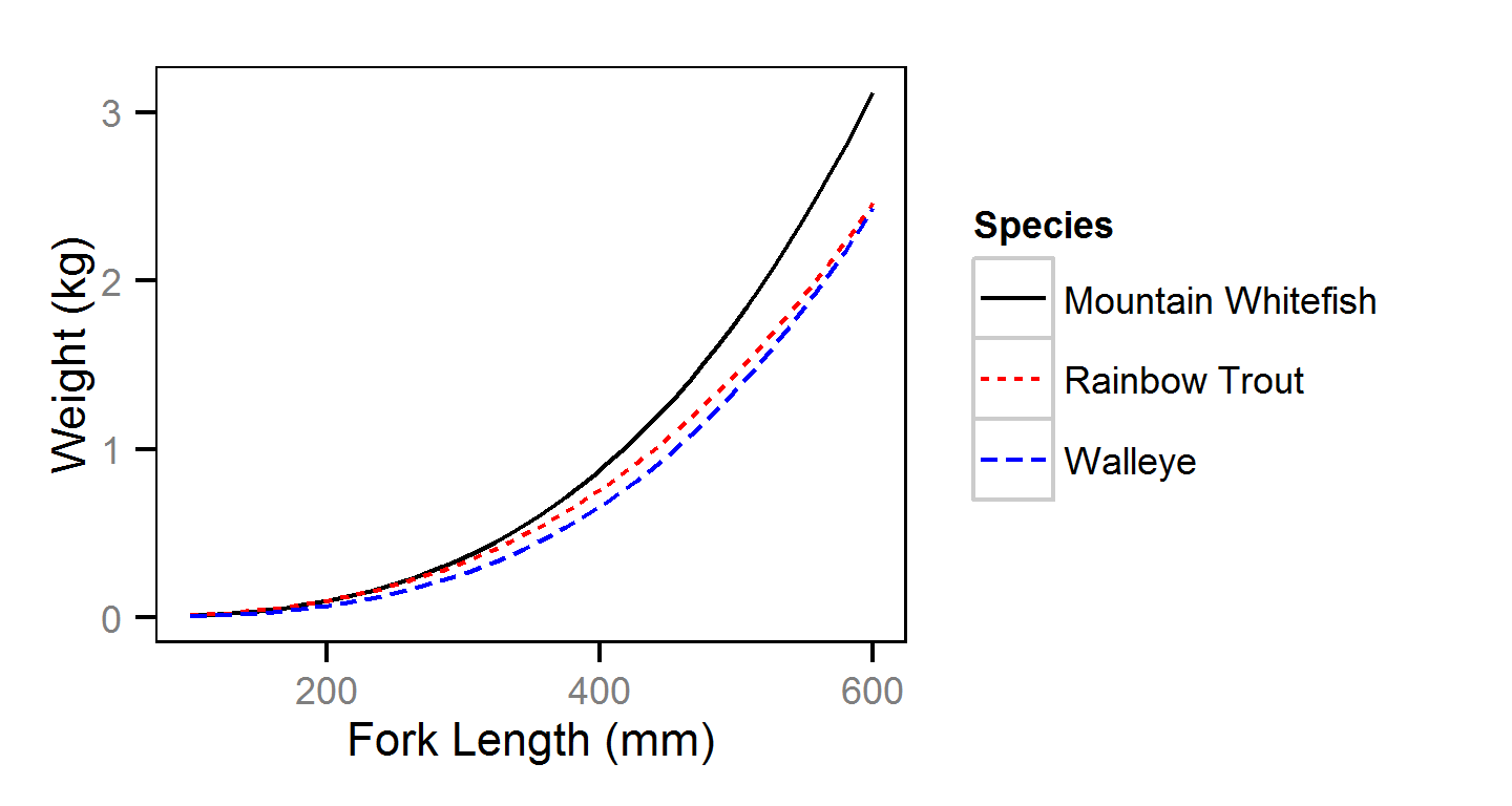
Figure 1. Predicted length-mass relationship by species.

Condition - Mountain Whitefish - Subadult

figures/condition/Subadult MW/year.png
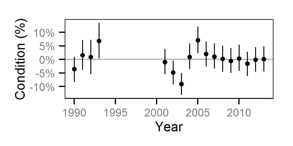
Figure 2. Predicted condition effect size for a 200 mm Mountain Whitefish by year (with 95% CRIs).

Condition - Mountain Whitefish - Adult

figures/condition/Adult MW/year.png
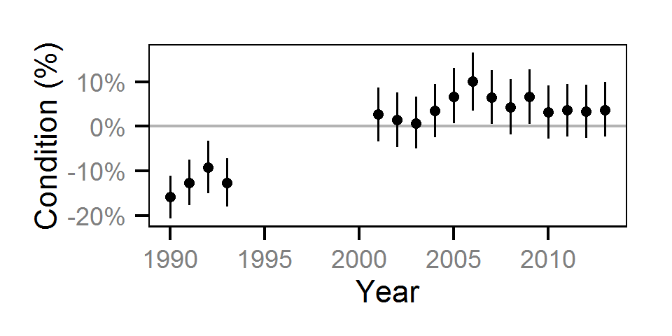
Figure 3. Predicted condition effect size for a 350 mm Mountain Whitefish by year (with 95% CRIs).

Condition - Rainbow Trout - Subadult

figures/condition/Subadult RB/year.png
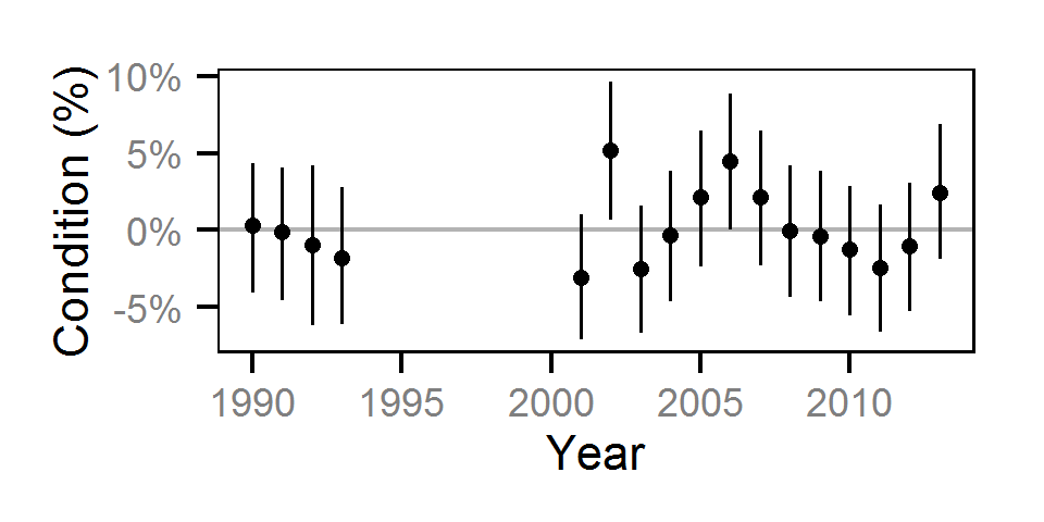
Figure 4. Predicted condition effect size for a 250 mm Rainbow Trout by year (with 95% CRIs).

Condition - Rainbow Trout - Adult

figures/condition/Adult RB/year.png
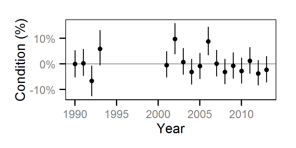
Figure 5. Predicted condition effect size for a 500 mm Rainbow Trout by year (with 95% CRIs).

Condition - Walleye - Adult

figures/condition/Adult WP/year.png
Figure 6. Predicted condition effect size for a 600 mm Walleye by year (with 95% CRIs).

Growth

figures/growth/growth.png
Figure 7. Predicted growth curve by species.

Growth - Mountain Whitefish

figures/growth/MW/year.png
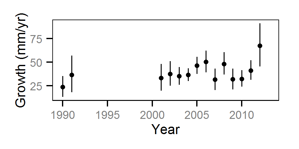
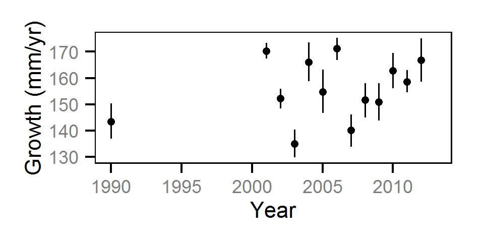
Figure 8. Predicted growth for a 200 mm Mountain Whitefish by year (with 95% CRIs).

Growth - Rainbow Trout

figures/growth/RB/year.png
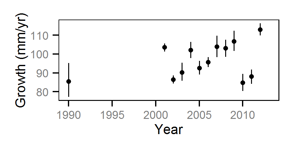
Figure 9. Predicted growth for a 200 mm Rainbow Trout by year (with 95% CRIs).

Growth - Walleye

figures/growth/WP/year.png
Figure 10. Predicted growth for a 200 mm Walleye by year (with 95% CRIs).

Length-At-Age - Mountain Whitefish - Age-0

figures/lengthatage/MW/Age-0/year.png
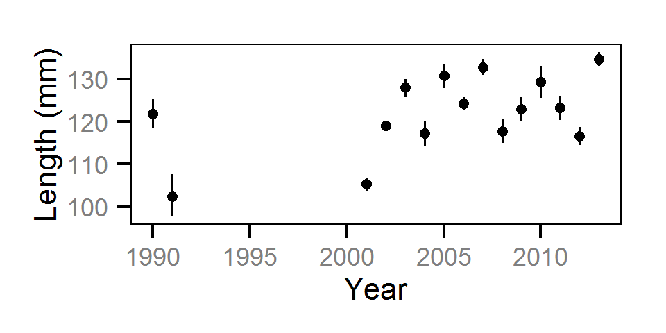
Figure 11. Predicted length of an age-0 Mountain Whitefish by year (with 95% CRIs).

Length-At-Age - Mountain Whitefish - Age-1

figures/lengthatage/MW/Age-1/year.png
Figure 12. Predicted growth of an age-0 (to age-1) Mountain Whitefish by year (with 95% CRIs).

Length-At-Age - Rainbow Trout - Age-0

figures/lengthatage/RB/Age-0/year.png
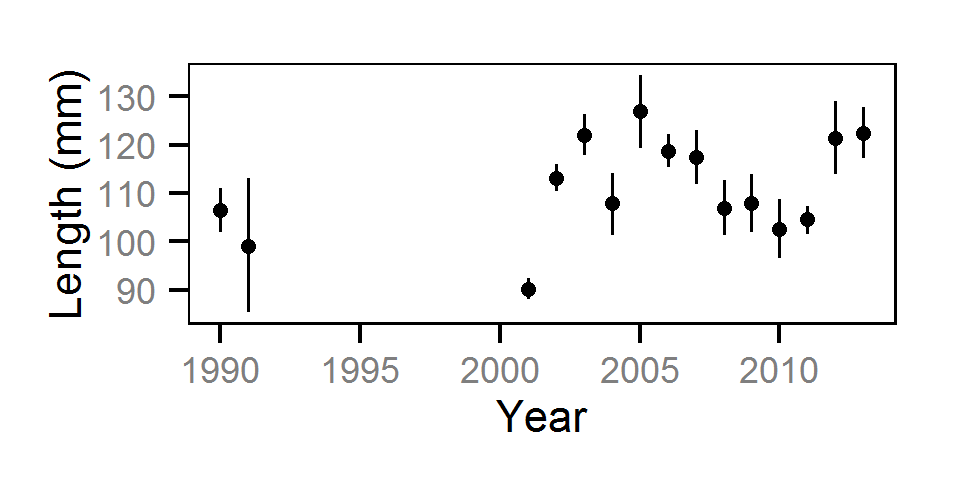
Figure 13. Predicted length of an age-0 Rainbow Trout by year (with 95% CRIs).

Length-At-Age - Rainbow Trout - Age-1

figures/lengthatage/RB/Age-1/year.png
Figure 14. Predicted growth of an age-0 (to age-1) Rainbow Trout by year (with 95% CRIs).

Length Bias

figures/observer/bias.png
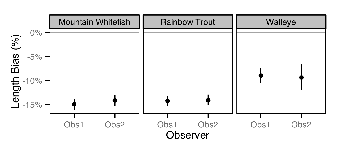
Figure 15. Predicted length bias by observer and species (with 95% CRIs).
figures/observer/density.png
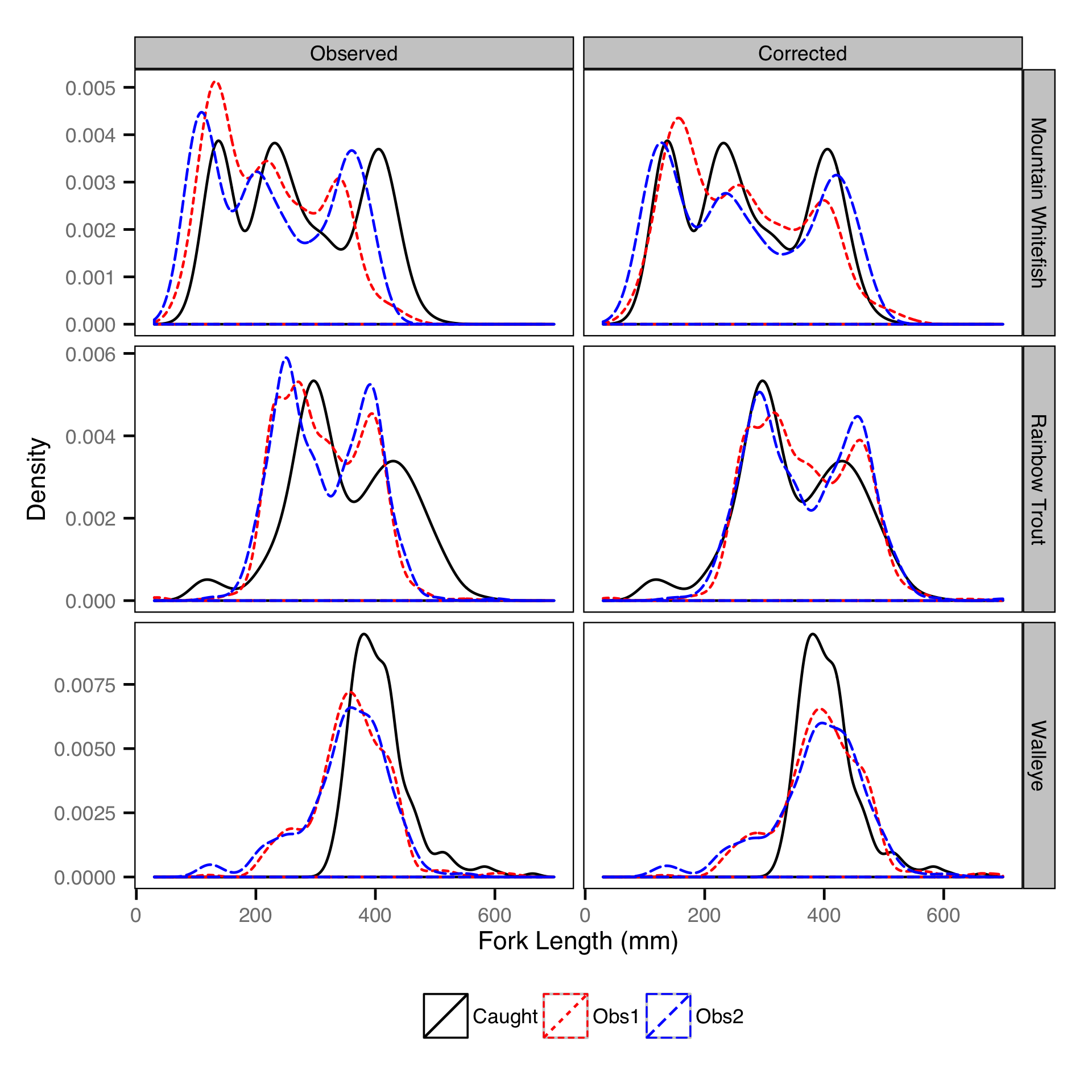
Figure 16. Observed and corrected length density plots for measured versus counted fish by observer and species.

Survival - Mountain Whitefish - Subadult

figures/survival/Subadult MW/year.png
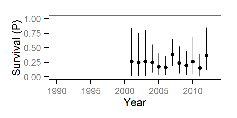
Figure 17. Predicted annual survival for a subadult Mountain Whitefish.

Survival - Mountain Whitefish - Adult

figures/survival/Adult MW/year.png
Figure 18. Predicted annual survival for an adult Mountain Whitefish.

Survival - Rainbow Trout - Subadult

figures/survival/Subadult RB/year.png
Figure 19. Predicted annual survival for a subadult Rainbow Trout.

Survival - Rainbow Trout - Adult

figures/survival/Adult RB/year.png
Figure 20. Predicted annual survival for an adult Rainbow Trout.

Survival - Walleye - Adult

figures/survival/Adult WP/year.png
Figure 21. Predicted annual survival for an adult Walleye.

Site Fidelity

figures/fidelity/length.png
Figure 22. Predicted site fidelity by species.

Capture Efficiency

figures/efficiency/efficiency.png
Figure 23. Predicted capture efficiency by species and life stage (with 95% CRIs).

Capture Efficiency - Mountain Whitefish - Subadult

figures/efficiency/Subadult MW/session-year.png
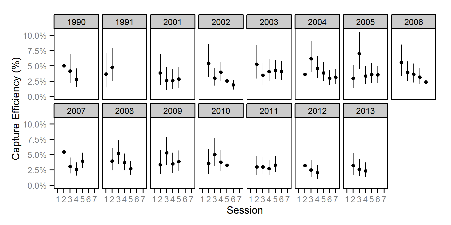
Figure 24. Predicted capture efficiency for a subadult Mountain Whitefish by session and year (with 95% CRIs).

Capture Efficiency - Mountain Whitefish - Adult

figures/efficiency/Adult MW/session-year.png
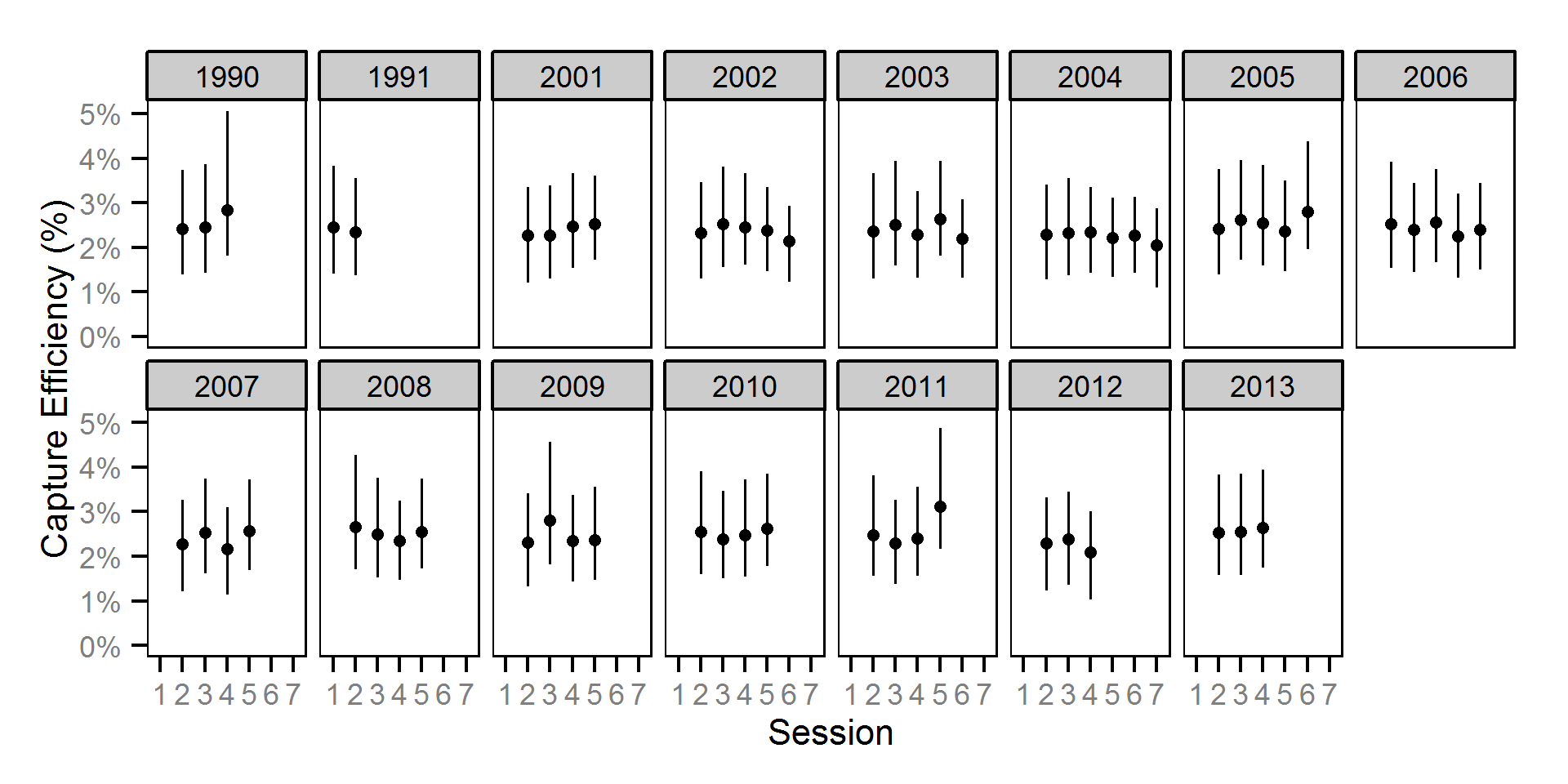
Figure 25. Predicted capture efficiency for an adult Mountain Whitefish by session and year (with 95% CRIs).

Capture Efficiency - Rainbow Trout - Subadult

figures/efficiency/Subadult RB/session-year.png
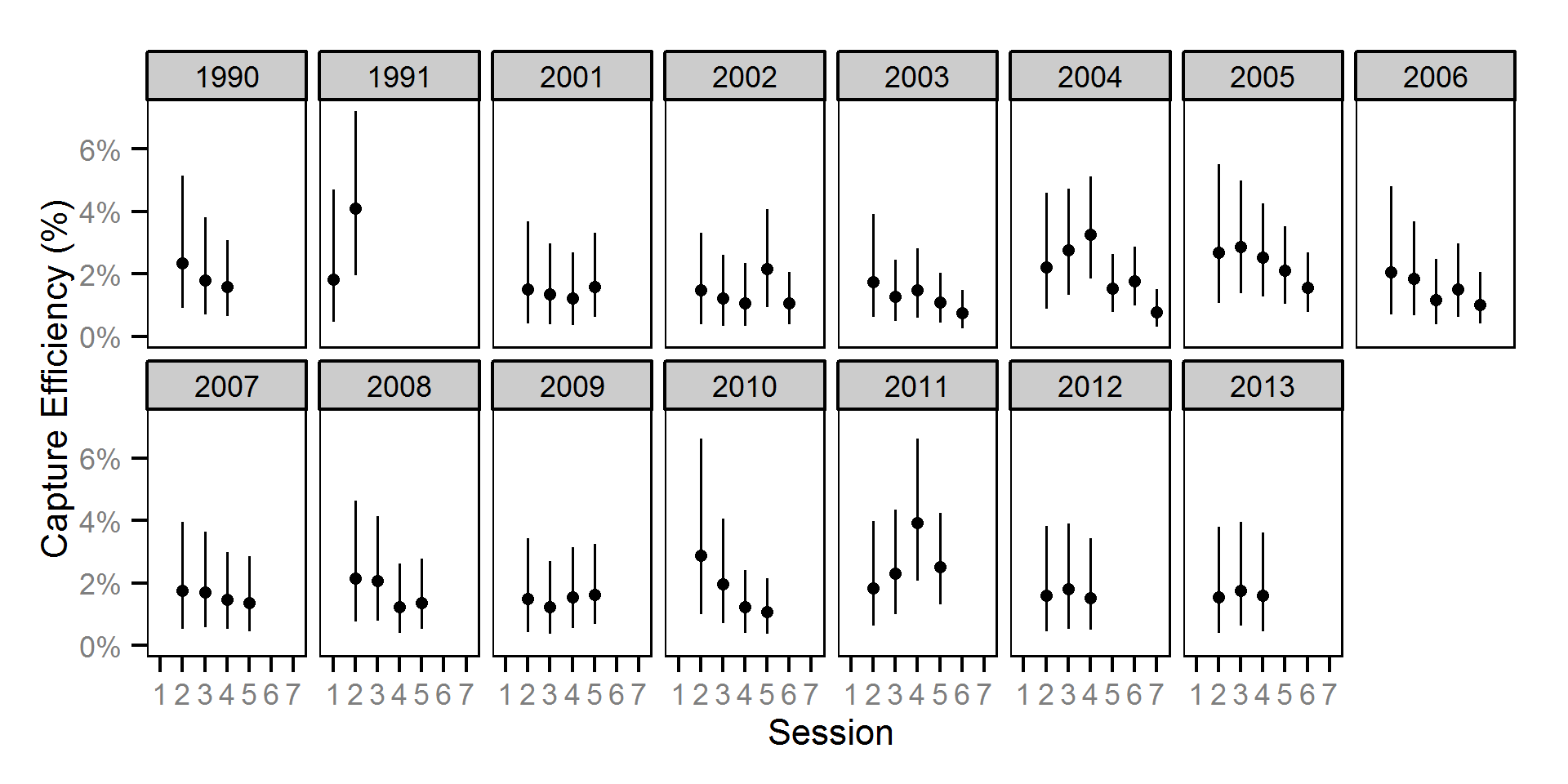
Figure 26. Predicted capture efficiency for a subadult Rainbow Trout by session and year (with 95% CRIs).

Capture Efficiency - Rainbow Trout - Adult

figures/efficiency/Adult RB/session-year.png
Figure 27. Predicted capture efficiency for an adult Rainbow Trout by session and year (with 95% CRIs).

Capture Efficiency - Walleye - Adult

figures/efficiency/Adult WP/session-year.png
Figure 28. Predicted capture efficiency for an adult Walleye by session and year (with 95% CRIs).

Abundance

figures/abundance/efficiency.png
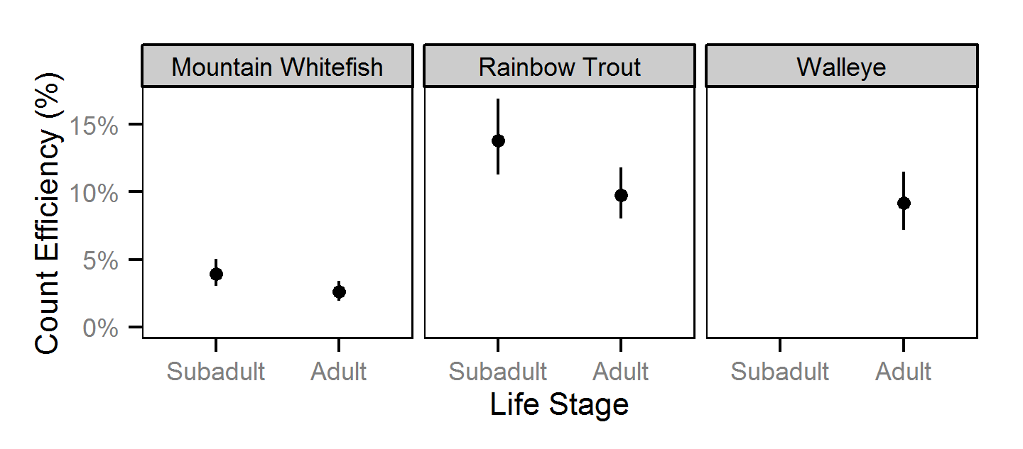
Figure 29. Predicted count efficiency by species and life stage (with 95% CRIs).
figures/abundance/count.png
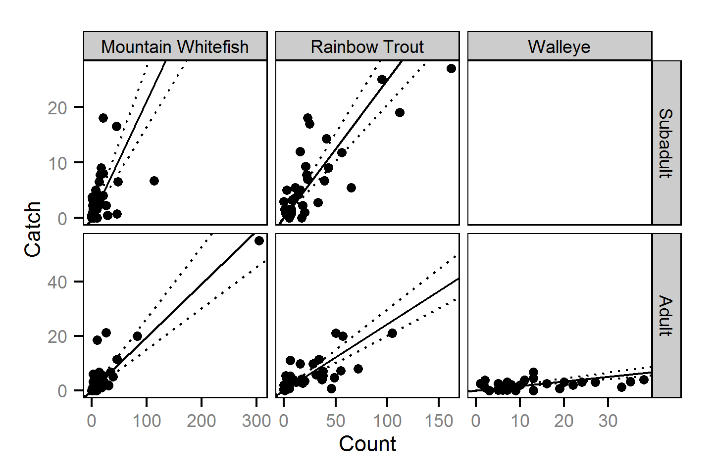
Figure 30. Predicted relationship between catch and count by species and life stage (with 95% CRIs) where the points are the mean site catches and counts for 2013.

Abundance - Mountain Whitefish - Subadult

figures/abundance/Subadult MW/year.png
Figure 31. Predicted abundance for subadult Mountain Whitefish by year (with 95% CRIs).
figures/abundance/Subadult MW/site.png
Figure 32. Predicted lineal channel density for subadult Mountain Whitefish by site (with 95% CRIs).

Abundance - Mountain Whitefish - Adult

figures/abundance/Adult MW/year.png
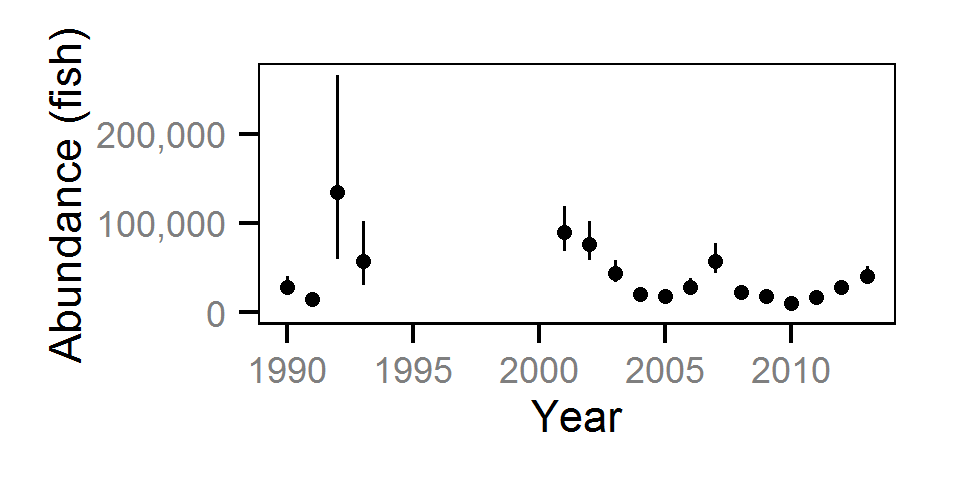
Figure 33. Predicted abundance for adult Mountain Whitefish by year (with 95% CRIs).
figures/abundance/Adult MW/site.png
Figure 34. Predicted lineal channel density for adult Mountain Whitefish by site (with 95% CRIs).

Abundance - Rainbow Trout - Subadult

figures/abundance/Subadult RB/year.png
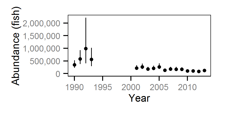
Figure 35. Predicted abundance for subadult Rainbow Trout by year (with 95% CRIs).
figures/abundance/Subadult RB/site.png
Figure 36. Predicted lineal channel density for subadult Rainbow Trout by site (with 95% CRIs).

Abundance - Rainbow Trout - Adult

figures/abundance/Adult RB/year.png
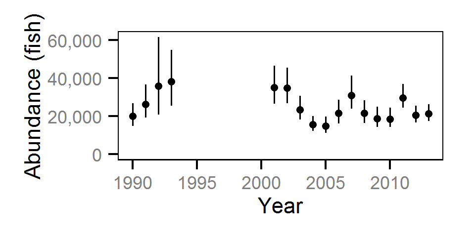
Figure 37. Predicted abundance for adult Rainbow Trout by year (with 95% CRIs).
figures/abundance/Adult RB/site.png
Figure 38. Predicted lineal channel density for adult Rainbow Trout by site (with 95% CRIs).

Abundance - Walleye - Adult

figures/abundance/Adult WP/year.png
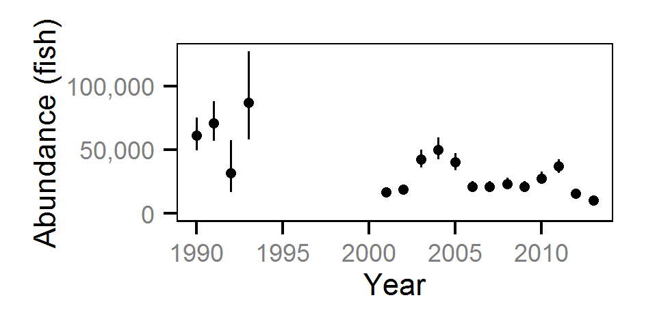
Figure 39. Predicted abundance for adult Walleye by year (with 95% CRIs).
figures/abundance/Adult WP/site.png
Figure 40. Predicted lineal channel density for adult Walleye by site (with 95% CRIs).

Dynamic Factor Analysis

figures/timeseries/observed.png
Figure 41. Environmental and fish index time series with DFA predicted values as black line (and 95% CRIs as dotted lines).
figures/timeseries/trends.png
Figure 42. Predicted DFA trend time series (with 95% CRIs).
figures/timeseries/weighting.png
Figure 43. Predicted DFA time series weightings by trend.
figures/timeseries/mds.png
Figure 44. Non-metric multidimensional plot showing clustering of time series based on the absolute DFA trend weightings.

Acknowledgements

The organisations and individuals whose contributions have made this analysis report possible include:

References

  • Michael Bradford, Josh Korman, Paul Higgins, (2005) Using confidence intervals to estimate the response of salmon populations (Oncorhynchus spp.) to experimental habitat alterations. Canadian Journal of Fisheries and Aquatic Sciences 62 (12) 2716-2726 10.1139/f05-179
  • A Fabens, (1965) Properties and fitting of the Von Bertalanffy growth curve. Growth 29 (3) 265-289
  • Hadley Wickham, (2009) ggplot2: elegant graphics for data analysis. http://had.co.nz/ggplot2/book
  • Ji He, James Bence, James Johnson, David Clapp, Mark Ebener, (2008) Modeling Variation in Mass-Length Relations and Condition Indices of Lake Trout and Chinook Salmon in Lake Huron: A Hierarchical Bayesian Approach. Transactions of the American Fisheries Society 137 (3) 801-817 10.1577/T07-012.1
  • Joseph Thorley, (2014) jaggernaut: An R package to facilitate Bayesian analyses using JAGS (Just Another Gibbs Sampler). https://github.com/joethorley/jaggernaut
  • Marc Kéry, Michael Schaub, (2011) Bayesian population analysis using {WinBUGS} : a hierarchical perspective. http://www.vogelwarte.ch/bpa.html
  • Martyn Plummer, (2012) {JAGS} version 3.3.0 user manual. http://sourceforge.net/projects/mcmc-jags/files/Manuals/3.x/
  • R Team, (2013) R: a language and environment for statistical computing. http://www.R-project.org
  • L. Bertalanffy, (1938) A quantitative theory of organic growth (inquiries on growth laws ii). Human Biology 10 181-213
  • A Zuur, I Tuck, N Bailey, (2003) Dynamic factor analysis to estimate common trends in fisheries time series. Canadian Journal of Fisheries and Aquatic Sciences 60 (5) 542-552 10.1139/f03-030