Duncan Lardeau Juvenile Rainbow Trout Abundance 2021
The suggested citation for this analytic report is:
Thorley, J.L., Andrusak, G.F. and Amies-Galonski, E. (2021) Duncan Lardeau Juvenile Rainbow Trout Abundance 2021. A Poisson Consulting Analytic Appendix. URL: https://www.poissonconsulting.ca/f/1275560691.
Background
Rainbow Trout rear in the Lardeau and Lower Duncan rivers. Since 2006 (with the exception of 2015) annual spring snorkel surveys have been conducted to estimate the abundance and distribution of age-1 Rainbow Trout. From 2006 to 2010 the surveys were conducted at fixed index sites. Since 2011 fish observations have been mapped to the river based on their spatial coordinates as recorded by GPS.
The primary aims of the current analyses were to:
- Estimate the spring abundance of age-1 fish by year.
- Estimate the egg deposition.
- Estimate the stock-recruitment relationship between the egg deposition and the abundance of age-1 recruits the following spring.
- Estimate the survival from age-1 to age-2.
- Estimate the expected number of spawners without in river and/or in lake variation.
Methods
Data Preparation
The data were provided by the Ministry of Forests, Lands and Natural Resource Operations (MFLNRO). The historical and current snorkel count data were manipulated using R version 4.1.0 (R Core Team 2021) and organised in an SQLite database.
Statistical Analysis
Model parameters were estimated using Bayesian methods. The estimates were produced using JAGS (Plummer 2003) and STAN (Carpenter et al. 2017). For additional information on Bayesian estimation the reader is referred to McElreath (2016), respectively.
Unless stated otherwise, the Bayesian analyses used weakly informative normal and half-normal prior distributions (Gelman et al. 2017). The posterior distributions were estimated from 1500 Markov Chain Monte Carlo (MCMC) samples thinned from the second halves of 3 chains (Kery and Schaub 2011, 38–40). Model convergence was confirmed by ensuring that the potential scale reduction factor \(\hat{R} \leq 1.05\) (Kery and Schaub 2011, 40) and the effective sample size (Brooks et al. 2011) \(\textrm{ESS} \geq 150\) for each of the monitored parameters (Kery and Schaub 2011, 61).
The parameters are summarised in terms of the point estimate, lower and upper 95% credible limits (CLs) and the surprisal s-value (Greenland 2019). The estimate is the median (50th percentile) of the MCMC samples while the 95% CLs are the 2.5th and 97.5th percentiles. The s-value can be considered a test of directionality. More specifically it indicates how surprising (in bits) it would be to discover that the true value of the parameter is in the opposite direction to the estimate. An s-value of 4.3 bits, which is equivalent to a p-value (Kery and Schaub 2011; Greenland and Poole 2013) of 0.05, indicates that the surprise would be equivalent to throwing 4.3 heads in a row.
The results are displayed graphically by plotting the modeled relationships between particular variables and the response(s) with the remaining variables held constant. In general, continuous and discrete fixed variables are held constant at their mean and first level values, respectively, while random variables are held constant at their typical values (expected values of the underlying hyperdistributions) (Kery and Schaub 2011, 77–82). When informative the influence of particular variables is expressed in terms of the effect size (i.e., percent or n-fold change in the response variable) with 95% credible intervals (CIs, Bradford et al. 2005).
The analyses were implemented using R version 4.1.0
(R Core Team 2021) and the
mbr family of packages.
Model Descriptions
Length Correction
The annual bias (inaccuracy) and error (imprecision) in observer’s fish length estimates when spotlighting (standing) and snorkeling were quantified from the divergence of their length distribution from the length distribution for all observers (including measured fish) in that year. More specifically, the length correction that minimised the Jensen-Shannon divergence (Lin 1991) between the two distributions provided a measure of the inaccuracy while the minimum divergence (the Jensen-Shannon divergence was calculated with log to base 2 which means it lies between 0 and 1) provided a measure of the imprecision.
After correcting the fish lengths, age-1 individuals were assumed to be those with a fork length \(\leq\) 100 mm.
Abundance
The abundance was estimated from the count data using an overdispersed Poisson model (Kery and Schaub 2011, 55–56). The annual abundance estimates represent the total number of fish in the study area.
Key assumptions of the abundance model include:
- The lineal fish density varies with year, useable width and river kilometer as a polynomial, and randomly with site.
- The observer efficiency at marking sites varies by study design (GPS versus Index).
- The observer efficiency also varies by visit type (marking versus count) within study design and randomly by snorkeller.
- The expected count at a site is the expected lineal density multiplied by the site length, the observer efficiency and the proportion of the site surveyed.
- The residual variation in the actual count is gamma-Poisson distributed.
Condition
The condition of fish with a fork length \(\geq\) 500 mm was estimated via an analysis of mass-length relations (He et al. 2008).
More specifically the model was based on the allometric relationship
\[ W = \alpha_c L^{\beta_c}\]
where \(W\) is the weight (mass), \(\alpha_c\) is the coefficent, \(\beta_c\) is the exponent and \(L\) is the length.
To improve chain mixing the relation was log-transformed, i.e.,
\[ \log(W) = \log(\alpha_c) + \beta_c \log(L).\]
Key assumptions of the condition model include:
- \(\alpha_c\) can vary randomly by year.
- The residual variation in weight is log-normally distributed.
Fecundity
The fecundity of females with a fork length \(\geq\) 500 mm was estimated via an analysis of fecundity-mass relations.
More specifically the model was based on the allometric relationship
\[ F = \alpha_f W^{\beta_f}\]
where \(F\) is the fecundity, \(\alpha_f\) is the coefficent, \(\beta_f\) is the exponent and \(W\) is the weight.
To improve chain mixing the relation was log-transformed.
Key assumptions of the fecundity model include:
- The residual variation in fecundity is log-normally distributed.
Spawner Size
The average length of the spawners in each year (for years for which it was unavailable) was estimated from the mean weight of Rainbow Trout in the Kootenay Lake Rainbow Trout Mailout Survey (KLRT) using a linear regression. This approach was suggested by Rob Bison.
Egg Deposition
The egg deposition in each year was estimated by
- converting the average length of spawners to the average weight using the condition relationship for a typical year
- adjusting the average weight by the annual condition effect (interpolating where unavailable)
- converting the average weight to the average fecundity using the fecundity relationship
- multiplying the average fecundity by the AUC based estimate of the number of females (assuming a sex ratio of 1:1)
Stock-Recruitment
The relationship between the number of eggs (\(E\)) and the abundance of age-1 individuals the following spring (\(R\)) was estimated using a Beverton-Holt stock-recruitment model (Walters and Martell 2004):
\[ R = \frac{\alpha_s \cdot E}{1 + \beta_s \cdot E} \quad,\]
where \(\alpha_s\) is the maximum number of recruits per egg (egg survival), and \(\beta_s\) is the density dependence.
Key assumptions of the stock-recruitment model include:
- The residual variation in the number of recruits is log-normally distributed with the standard deviation scaling with the uncertainty in the number of recruits.
The age-1 carrying capacity (\(K\)) is given by:
\[ K = \frac{\alpha_s}{\beta_s} \quad.\]
and the \(E_{K/2}\) Limit Reference Point (Mace 1994, \(E_{0.5 R_{max}}\)), which corresponds to the stock (number of eggs) that produce 50% of the maximum recruitment (\(K\)), by \[E_{K/2} = \frac{1}{\beta_s}\]
The LRP was also converted into a number of spawners in a typical year (assuming 6,000 eggs per spawner and a sex ratio of 1:1).
Age-1 to Age-2 Survival
The relationship between the number of age-1 individuals and the number of age-2 individuals the following year was estimated using a linear regression through the origin where the slope was constrained to lie between 0 and 1 by a logistic transformation.
Key assumptions of the survival rate model include:
- The residual variation in the number of age-2 individuals is log-normally distributed.
Reproductive Rate
The maximum reproductive rate (the number of spawners per spawner at low density) not accounting for fishing mortality was calculated by multiplying \(\beta_s\) (number of recruits per egg at low density) from the stock-recruitment relationship by the inlake survival by the estimated eggs per spawner in each year (assuming a sex ratio of 1:1). The inlake survival from age-1 to spawning was calculated by dividing the subsequent number of spawners by the number of recruits assuming that equal numbers of fish spawn at age 5, 6 and 7.
Expected Spawners
The expected spawners without in river and/or in lake variation was calculated from the stock-recruitment relationship and assuming an age-1 to spawner survival of 0.68%.
Results
Model Templates
Abundance
  data {

    int<lower=0> nMarked;
    int<lower=0> Marked[nMarked];
    int<lower=0> Resighted[nMarked];
    int<lower=0> IndexMarked[nMarked];

    int<lower=0> nObs;
    int Marking[nObs];
    int Index[nObs];
    int<lower=0> nSwimmer;
    int<lower=0> Swimmer[nObs];
    int<lower=0> nYear;
    int<lower=0> Year[nObs];
    real Rkm[nObs];
    int<lower=0> nSite;
    int<lower=0> Site[nObs];

    real SiteLength[nObs];
    real SurveyProportion[nObs];

    int Count[nObs];
  }
  parameters {
    real bEfficiency;
    real bEfficiencyIndex;

    real bDensity;
    real<lower=0> sDensityYear;
    vector[nYear] bDensityYear;

    vector[4] bDensityRkm;
    real<lower=0> sDensitySite;
    vector[nSite] bDensitySite;

    real bEfficiencyMarking;
    real bEfficiencyMarkingIndex;

    real<lower=0,upper=5> sEfficiencySwimmer;
    vector[nSwimmer] bEfficiencySwimmer;

    real<lower=0> sDispersion;
  }
  model {

    vector[nObs] eDensity;
    vector[nObs] eEfficiency;
    vector[nObs] eAbundance;
    vector[nObs] eCount;

    sDispersion ~ gamma(0.01, 0.01);

    bDensity ~ normal(0, 2);
    bDensityRkm ~ normal(0, 2);
    sDensitySite ~ uniform(0, 5);
    bDensitySite ~ normal(0, sDensitySite);
    sDensityYear ~ uniform(0, 5);
    bDensityYear ~ normal(0, sDensityYear);

    bEfficiency ~ normal(0, 5);
    bEfficiencyIndex ~ normal(0, 5);
    bEfficiencyMarking ~ normal(0, 5);
    bEfficiencyMarkingIndex ~ normal(0, 5);
    sEfficiencySwimmer ~ uniform(0, 5);
    bEfficiencySwimmer ~ normal(0, sEfficiencySwimmer);

    for (i in 1:nMarked) {
      target += binomial_lpmf(Resighted[i] | Marked[i],
        inv_logit(
          bEfficiency +
          bEfficiencyIndex * IndexMarked[i] +
          bEfficiencyMarking +
          bEfficiencyMarkingIndex * IndexMarked[i]
        ));
    }

    for (i in 1:nObs) {
      eDensity[i] = exp(bDensity +
                        bDensityRkm[1] * Rkm[i] +
                        bDensityRkm[2] * pow(Rkm[i], 2.0) +
                        bDensityRkm[3] * pow(Rkm[i], 3.0) +
                        bDensityRkm[4] * pow(Rkm[i], 4.0) +
                        bDensitySite[Site[i]] +
                        bDensityYear[Year[i]]);

      eEfficiency[i] = inv_logit(
        bEfficiency +
        bEfficiencyIndex * Index[i] +
        bEfficiencyMarking * Marking[i] +
        bEfficiencyMarkingIndex * Index[i] * Marking[i] +
        bEfficiencySwimmer[Swimmer[i]]);

      eAbundance[i] = eDensity[i] * SiteLength[i];

      eCount[i] = eAbundance[i] * eEfficiency[i] * SurveyProportion[i];
    }

    target += neg_binomial_2_lpmf(Count | eCount, sDispersion);
  }
Block 1. Abundance model description.
Condition
 data {
  int nYear;
  int nObs;

  vector[nObs] Length;
  vector[nObs] Weight;
  int Year[nObs];

parameters {
  real bWeight;
  real bWeightLength;
  real sWeightYear;

  vector[nYear] bWeightYear;
  real sWeight;

model {

  vector[nObs] eWeight;

  bWeight ~ normal(-10, 5);
  bWeightLength ~ normal(3, 2);

  sWeightYear ~ normal(-2, 5);

  for (i in 1:nYear) {
    bWeightYear[i] ~ normal(0, exp(sWeightYear));
  }

  sWeight ~ normal(-2, 5);
  for(i in 1:nObs) {
    eWeight[i] = bWeight + bWeightLength * log(Length[i]) + bWeightYear[Year[i]];
    Weight[i] ~ lognormal(eWeight[i], exp(sWeight));
  }
Block 2.
Fecundity
 data {
  int nObs;

  vector[nObs] Weight;
  vector[nObs] Fecundity;

parameters {
  real bFecundity;
  real bFecundityWeight;
  real sFecundity;

model {

  vector[nObs] eFecundity;

  bFecundity ~ uniform(0, 5);
  bFecundityWeight ~ uniform(0, 2);

  sFecundity ~ uniform(0, 1);
  for(i in 1:nObs) {
    eFecundity[i] = log(bFecundity) + bFecundityWeight * log(Weight[i]);
    Fecundity[i] ~ lognormal(eFecundity[i], sFecundity);
  }
Block 3.
Stock-Recruitment
model {
  a ~ dunif(0, 1)
  b ~ dunif(0, 0.1)
  sScaling ~ dunif(0, 5)

  eRecruits <- a * Stock / (1 + Stock * b)

  for(i in 1:nObs) {
    esRecruits[i] <- SDLogRecruits[i] * sScaling
    Recruits[i] ~ dlnorm(log(eRecruits[i]), esRecruits[i]^-2)
  }
Block 4. Stock-Recruitment model description.
Age-1 to Age-2 Survival
model {
  bSurvival ~ dnorm(0, 2^-2)
  sRecruits ~ dnorm(0, 2^-2) T(0,)

  for(i in 1:nObs) {
    logit(eSurvival[i]) <- bSurvival
    eRecruits[i] <- Stock[i] * eSurvival[i]
    Recruits[i] ~ dlnorm(log(eRecruits[i]), sRecruits^-2)
  }
Block 5. In-river survival model description.
Tables
Abundance
Table 1. Parameter descriptions.
| Parameter | Description |
|---|---|
bDensity |
Intercept for log(eDensity) |
bDensityRkm[i] |
ith-order polynomial coefficients of effect of
river kilometer on bDensity |
bDensitySite[i] |
Effect of ith Site on bDensity |
bDensityYear[i] |
Effect of ith Year on bDensity |
bEfficiency |
Intercept of logit(eEfficiency) |
bEfficiencyIndex |
Effect of Index on bEfficiency |
bEfficiencyMarking |
Effect of Marking on bEfficiency |
bEfficiencyMarkingIndex |
Effect of Marking and Index on bEfficiency |
bEfficiencySwimmer[i] |
Effect of ith Swimmer on bEfficiency |
eAbundance[i] |
Expected abundance of fish at site of ith visit |
eCount[i] |
Expected total number of fish at site of ith
visit |
eDensity[i] |
Expected lineal density of fish at site of ith
visit |
eEfficiency[i] |
Expected observer efficiency on ith visit |
Index |
Whether the ith visit was to an index site |
Marking[i] |
Whether the ith visit was to a site with marked
fish |
Rkm[i] |
River kilometer of ith visit |
sDensitySite |
SD of bDensitySite |
sDispersion |
Overdispersion of Count[i] |
sEfficiencySwimmer |
SD of bEfficiencySwimmer |
Site[i] |
Site of ith visit |
SiteLength[i] |
Length of site of ith visit |
SurveyProportion[i] |
Proportion of site surveyed on ith visit |
Swimmer[i] |
Snorkeler on ith site visit |
Year[i] |
Year of ith site visit |
Age-1
Table 2. Model coefficients.
| term | estimate | lower | upper | svalue |
|---|---|---|---|---|
| bDensity | -1.2098091 | -1.6747048 | -0.6972998 | 10.551708 |
| bDensityRkm[1] | -0.1927617 | -0.3440534 | -0.0359800 | 6.303781 |
| bDensityRkm[2] | 0.5900044 | 0.3786136 | 0.7952371 | 10.551708 |
| bDensityRkm[3] | -0.1132496 | -0.1922307 | -0.0411864 | 8.966746 |
| bDensityRkm[4] | -0.2771688 | -0.3516006 | -0.2055780 | 10.551708 |
| bEfficiency | -1.8013903 | -2.0749370 | -1.5160279 | 10.551708 |
| bEfficiencyIndex | 0.3369932 | -0.2483043 | 0.9882405 | 1.840902 |
| bEfficiencyMarking | 0.4952944 | 0.2727450 | 0.7038776 | 10.551708 |
| bEfficiencyMarkingIndex | 0.9203477 | 0.2690139 | 1.5397472 | 7.092277 |
| sDensitySite | 0.6610888 | 0.5943993 | 0.7335773 | 10.551708 |
| sDensityYear | 0.6717474 | 0.4612568 | 1.0363068 | 10.551708 |
| sDispersion | 1.3056903 | 1.1739344 | 1.4479836 | 10.551708 |
| sEfficiencySwimmer | 0.4678608 | 0.2768795 | 0.8591817 | 10.551708 |
Table 3. Model summary.
| n | K | nchains | niters | nthin | ess | rhat | converged |
|---|---|---|---|---|---|---|---|
| 3508 | 13 | 3 | 500 | 5 | 759 | 1.007 | TRUE |
Table 4. Model posterior predictive checks.
| moment | observed | median | lower | upper | svalue |
|---|---|---|---|---|---|
| zeros | 0.0000000 | 0.0000000 | 0.0000000 | 0.0000000 | 0.00000 |
| mean | -0.3005236 | -0.3681359 | -0.4018284 | -0.3352433 | 10.55171 |
| variance | 0.6007891 | 0.8558667 | 0.8133539 | 0.8987680 | 10.55171 |
| skewness | 0.1858572 | 0.5375591 | 0.4573260 | 0.6230798 | 10.55171 |
| kurtosis | -0.5426561 | -0.1995929 | -0.3723576 | 0.0247367 | 10.55171 |
Age-2
Table 5. Model coefficients.
| term | estimate | lower | upper | svalue |
|---|---|---|---|---|
| bDensity | -2.0842028 | -2.5926068 | -1.5915817 | 10.5517083 |
| bDensityRkm[1] | -0.2128592 | -0.4130666 | -0.0334140 | 5.3422549 |
| bDensityRkm[2] | 0.0336427 | -0.2243816 | 0.2757409 | 0.3265008 |
| bDensityRkm[3] | 0.0425520 | -0.0489595 | 0.1355835 | 1.5601864 |
| bDensityRkm[4] | -0.0945494 | -0.1781345 | -0.0060137 | 5.0598552 |
| bEfficiency | -2.0329898 | -2.4692558 | -1.5949384 | 10.5517083 |
| bEfficiencyIndex | 0.5349712 | -0.1192730 | 1.2363483 | 3.2029801 |
| bEfficiencyMarking | 0.7176875 | 0.3992786 | 1.0513500 | 10.5517083 |
| bEfficiencyMarkingIndex | 2.1668745 | 1.1393489 | 3.2477195 | 10.5517083 |
| sDensitySite | 0.7740179 | 0.6865336 | 0.8684278 | 10.5517083 |
| sDensityYear | 0.5460727 | 0.3690789 | 0.8834438 | 10.5517083 |
| sDispersion | 1.1716236 | 1.0111061 | 1.3885311 | 10.5517083 |
| sEfficiencySwimmer | 0.3873169 | 0.2325397 | 0.6511071 | 10.5517083 |
Table 6. Model summary.
| n | K | nchains | niters | nthin | ess | rhat | converged |
|---|---|---|---|---|---|---|---|
| 3508 | 13 | 3 | 500 | 5 | 768 | 1.009 | TRUE |
Table 7. Model posterior predictive checks.
| moment | observed | median | lower | upper | svalue |
|---|---|---|---|---|---|
| zeros | 0.0000000 | 0.0000000 | 0.0000000 | 0.0000000 | 0.0009615 |
| mean | -0.3093311 | -0.3362331 | -0.3670306 | -0.3078566 | 3.7835239 |
| variance | 0.5801792 | 0.7274513 | 0.6770241 | 0.7744862 | 10.5517083 |
| skewness | 0.7303687 | 0.8791963 | 0.7842122 | 0.9798257 | 10.5517083 |
| kurtosis | -0.1378032 | 0.3223071 | 0.0477461 | 0.6584863 | 10.5517083 |
Condition
Table 8. Parameter descriptions.
| Parameter | Description |
|---|---|
bWeight |
Intercept of log(eWeight) |
bWeightLength |
Intercept of effect of log(Length) on bWeight |
bWeightYear[i] |
Effect of ith Year on bWeight |
eWeight[i] |
Expected Weight of ith fish |
Length[i] |
Fork length of ith fish |
sWeight |
Log standard deviation of residual variation in log(Weight) |
sWeightYear |
Log standard deviation of bWeightYear |
Weight[i] |
Recorded weight of ith fish |
Year[i] |
Year ith fish was captured |
Table 9. Model coefficients.
| term | estimate | lower | upper | svalue |
|---|---|---|---|---|
| bWeight | -8.957515 | -9.577279 | -8.327107 | 10.55171 |
| bWeightLength | 2.636533 | 2.540749 | 2.729346 | 10.55171 |
| sWeight | -1.412853 | -1.451705 | -1.369734 | 10.55171 |
| sWeightYear | -1.593725 | -1.897886 | -1.251610 | 10.55171 |
Table 10. Model summary.
| n | K | nchains | niters | nthin | ess | rhat | converged |
|---|---|---|---|---|---|---|---|
| 1185 | 4 | 3 | 500 | 2 | 304 | 1.005 | TRUE |
Table 11. Model posterior predictive checks.
| moment | observed | median | lower | upper | svalue |
|---|---|---|---|---|---|
| zeros | 0.0000000 | 0.0000000 | 0.0000000 | 0.0000000 | 0.0000000 |
| mean | 0.0007358 | -0.0017763 | -0.0831461 | 0.0801327 | 0.0851219 |
| variance | 1.9582756 | 2.0009886 | 1.8506364 | 2.1637770 | 0.7235718 |
| skewness | -11.6566714 | -0.0012152 | -0.1455530 | 0.1380060 | 10.5517083 |
| kurtosis | 287.3216012 | -0.0043032 | -0.2486362 | 0.3319438 | 10.5517083 |
Table 12. Model sensitivity.
| n | K | nchains | niters | rhat_1 | rhat_2 | rhat_all | converged |
|---|---|---|---|---|---|---|---|
| 1185 | 4 | 3 | 500 | 1.005 | 1.008 | 1.004 | TRUE |
Fecundity
Table 13. Parameter descriptions.
| Parameter | Description |
|---|---|
bFecundity |
Intercept of eFecundity |
bFecundityWeight |
Effect of log(Weight) on log(bFecundity) |
eFecundity[i] |
Expected Fecundity of ith fish |
Fecundity[i] |
Fecundity of ith fish (eggs) |
sFecundity |
SD of residual variation in log(Fecundity) |
Weight[i] |
Weight of ith fish (mm) |
Table 14. Model coefficients.
| term | estimate | lower | upper | svalue |
|---|---|---|---|---|
| bFecundity | 3.8649273 | 1.4275232 | 4.9500189 | 10.55171 |
| bFecundityWeight | 0.8610988 | 0.8317531 | 0.9739412 | 10.55171 |
| sFecundity | 0.1273735 | 0.0932693 | 0.1865299 | 10.55171 |
Table 15. Model summary.
| n | K | nchains | niters | nthin | ess | rhat | converged |
|---|---|---|---|---|---|---|---|
| 22 | 3 | 3 | 500 | 2 | 262 | 1.016 | TRUE |
Table 16. Model posterior predictive checks.
| moment | observed | median | lower | upper | svalue |
|---|---|---|---|---|---|
| zeros | 0.0000000 | 0.0000000 | 0.0000000 | 0.0000000 | 0.0000000 |
| mean | 0.0145273 | 0.0117784 | -0.5468271 | 0.5663281 | 0.0077098 |
| variance | 1.8242731 | 1.9354759 | 0.9661501 | 3.4151509 | 0.2536457 |
| skewness | -2.1200692 | 0.0162370 | -0.9750692 | 0.9409571 | 10.5517083 |
| kurtosis | 6.5274329 | -0.4055770 | -1.2334752 | 1.9683889 | 8.9667458 |
Table 17. Model sensitivity.
| n | K | nchains | niters | rhat_1 | rhat_2 | rhat_all | converged |
|---|---|---|---|---|---|---|---|
| 22 | 3 | 3 | 500 | 1.016 | 1.006 | 1.01 | TRUE |
Stock-Recruitment
Table 18. Parameter descriptions.
| Parameter | Description |
|---|---|
a |
Recruits per Stock at low density |
b |
Density-dependence |
eRecruits[i] |
Expected number of recruits from ith spawn year |
esRecruits[i] |
Expected SD of residual variation in Recruits |
Recruits[i] |
Number of recruits from ith spawn year |
SDLogRecruits[i] |
Standard deviation of uncertainty in log(Recruits[i]) |
sScaling |
Scaling term for SD of residual variation in log(eRecruits) |
Stock[i] |
Number of egg in ith spawn year |
Age-1
Table 19. Model coefficients.
| term | estimate | lower | upper | svalue |
|---|---|---|---|---|
| a | 0.4838583 | 0.2211006 | 0.9626915 | 10.55171 |
| b | 0.0000046 | 0.0000015 | 0.0000116 | 10.55171 |
| sScaling | 2.4329909 | 1.6894008 | 3.9092801 | 10.55171 |
Table 20. Model summary.
| n | K | nchains | niters | nthin | ess | rhat | converged |
|---|---|---|---|---|---|---|---|
| 15 | 3 | 3 | 500 | 100 | 1264 | 1.001 | TRUE |
Table 21. Estimated carry capacity (with 95% CRIs).
| estimate | lower | upper |
|---|---|---|
| 104000 | 70400 | 165000 |
Table 22. Model posterior predictive checks.
| moment | observed | median | lower | upper | svalue |
|---|---|---|---|---|---|
| zeros | 0.0000000 | 0.0000000 | 0.0000000 | 0.0000000 | 0.0000000 |
| mean | -0.0303758 | 0.0317910 | -0.6874105 | 0.7585917 | 0.1690842 |
| variance | 9.9527274 | 1.9560945 | 0.8217253 | 3.7740285 | 10.5517083 |
| skewness | 0.0010579 | -0.0071256 | -1.0580164 | 1.0567720 | 0.0271665 |
| kurtosis | -0.7404681 | -0.5417368 | -1.3705987 | 1.6298662 | 0.3805315 |
Table 23. Estimated reference points (with 80% CRIs).
| Metric | estimate | lower | upper |
|---|---|---|---|
| eggs | 218000.00000 | 106000.00000 | 471000 |
| spawners | 72.66667 | 35.33333 | 157 |
Table 24. Model sensitivity.
| n | K | nchains | niters | rhat_1 | rhat_2 | rhat_all | converged |
|---|---|---|---|---|---|---|---|
| 15 | 3 | 3 | 500 | 1.001 | 1.003 | 1.001 | TRUE |
Age-1 to Age-2 Survival
Table 25. Parameter descriptions.
| Parameter | Description |
|---|---|
bSurvival |
logit(eSurvival) |
eSurvival[i] |
Expected annual survival for ith spawn year |
Recruits[i] |
Number of age-2 juveniles from ith spawn year |
sRecruits |
SD of residual variation in Recruits |
Stock[i] |
Number of age-1 juveniles from ith spawn year |
Age-2
Table 26. Model coefficients.
| term | estimate | lower | upper | svalue |
|---|---|---|---|---|
| bSurvival | -0.8812839 | -1.2203869 | -0.506210 | 7.092277 |
| sRecruits | 0.4343028 | 0.2979112 | 0.713525 | 10.551708 |
Table 27. Model summary.
| n | K | nchains | niters | nthin | ess | rhat | converged |
|---|---|---|---|---|---|---|---|
| 13 | 2 | 3 | 500 | 1 | 555 | 1.006 | TRUE |
Table 28. Model posterior predictive checks.
| moment | observed | median | lower | upper | svalue |
|---|---|---|---|---|---|
| zeros | 0.0000000 | 0.0000000 | 0.0000000 | 0.0000000 | 0.0000000 |
| mean | -0.0467403 | -0.0029952 | -0.8161317 | 0.7575169 | 0.1202107 |
| variance | 1.7252479 | 1.8310607 | 0.7654493 | 3.7019920 | 0.1821109 |
| skewness | -0.1959049 | 0.0110819 | -1.0891284 | 1.0667994 | 0.5446810 |
| kurtosis | -1.2697298 | -0.6210505 | -1.3920507 | 1.4292329 | 2.8169986 |
Table 29. Model sensitivity.
| n | K | nchains | niters | rhat_1 | rhat_2 | rhat_all | converged |
|---|---|---|---|---|---|---|---|
| 13 | 2 | 3 | 500 | 1.006 | 1.003 | 1.004 | TRUE |
Figures
Length Correction
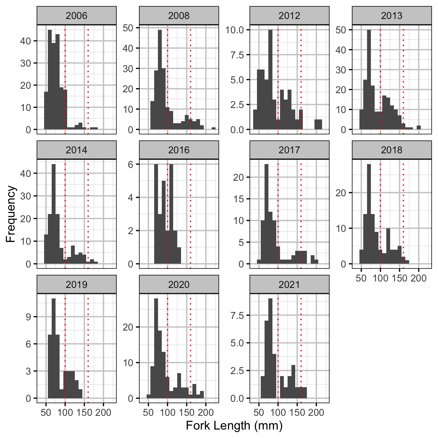
Figure 1. Measured length-frequency histogram by year.
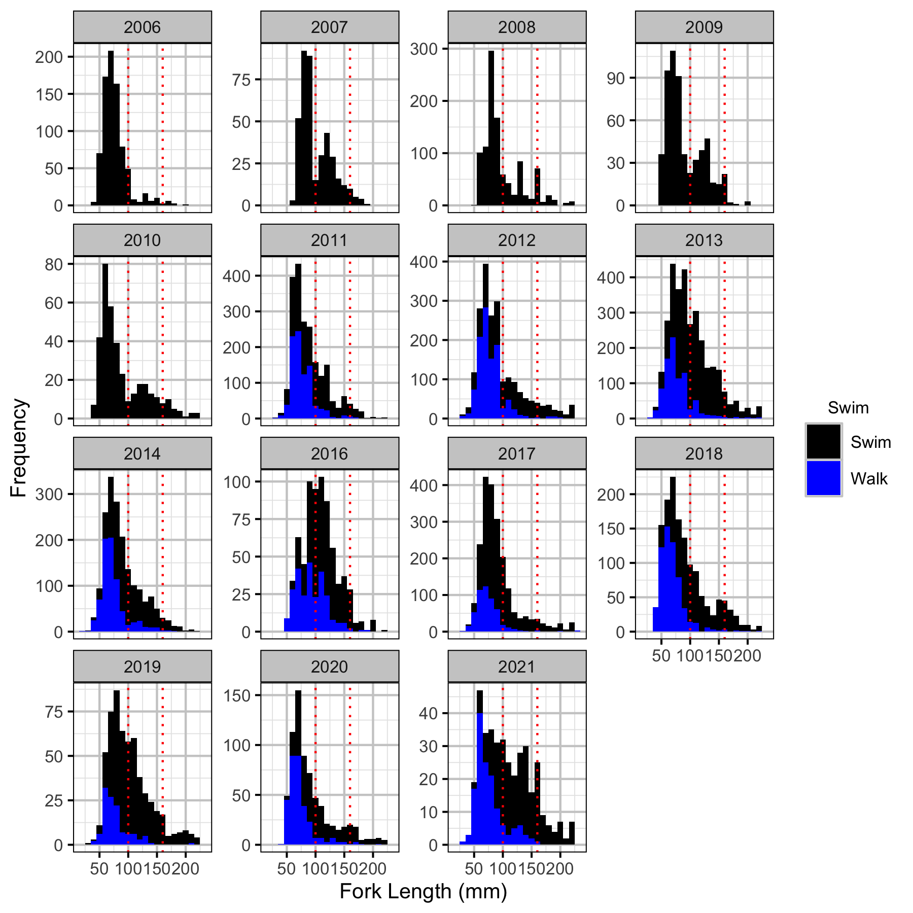
Figure 2. Corrected length-frequency histogram by year and observation type.
Abundance
Age-1
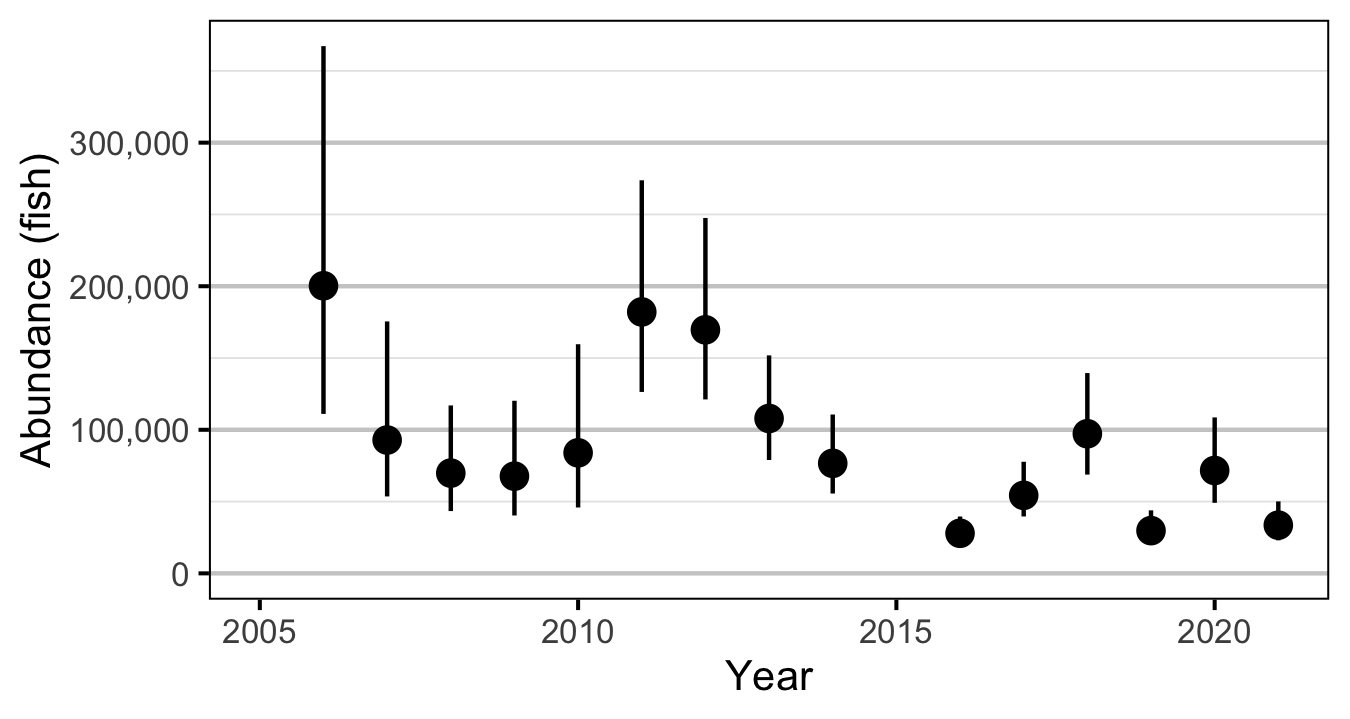
Figure 3. Predicted abundance of age-1 Rainbow Trout in the Duncan and Lardeau Rivers by year (with 95% CRIs).
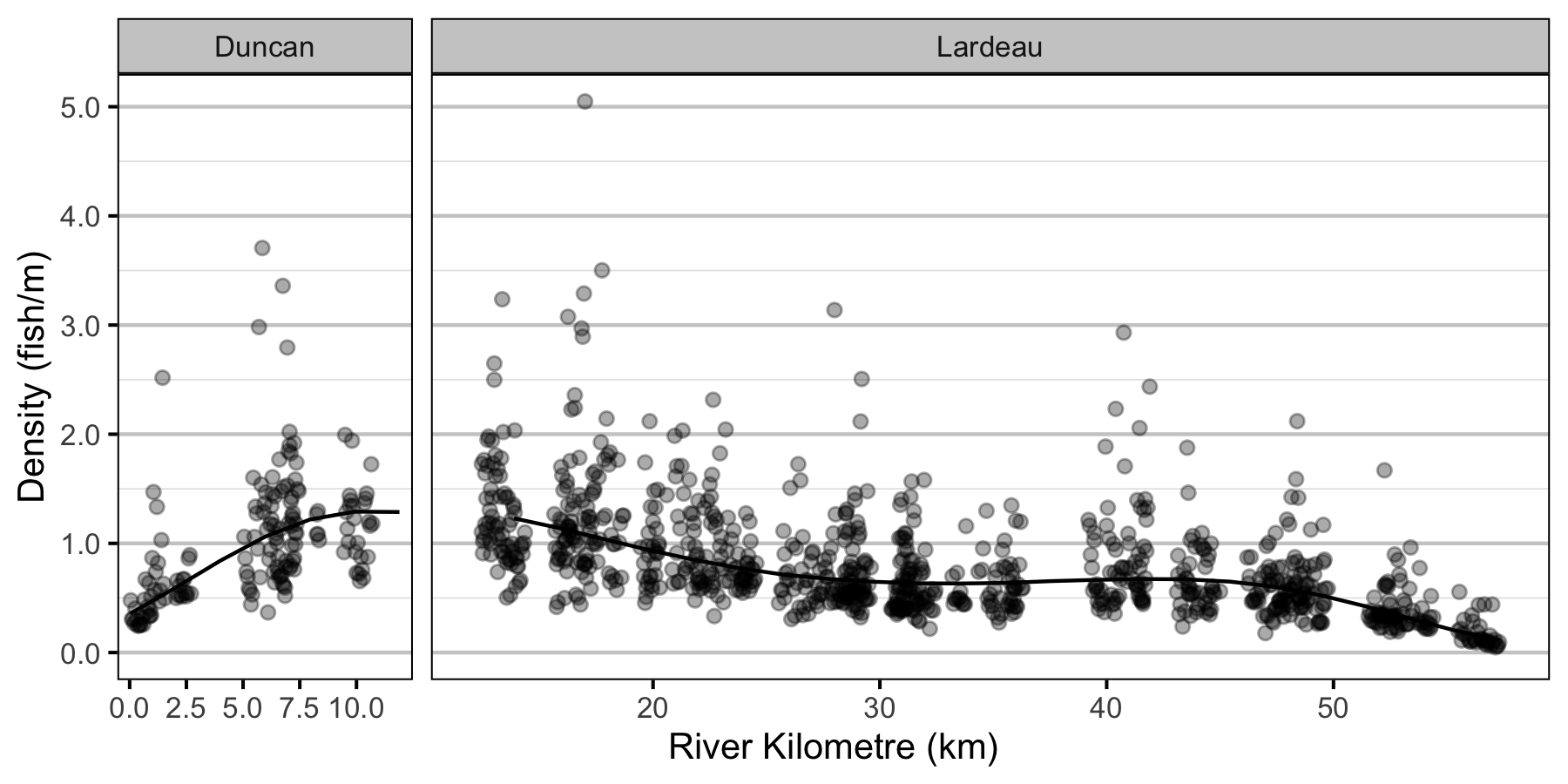
Figure 4. Predicted lineal density of age-1 Rainbow Trout in 2010 by river kilometre (with 95% CRIs).
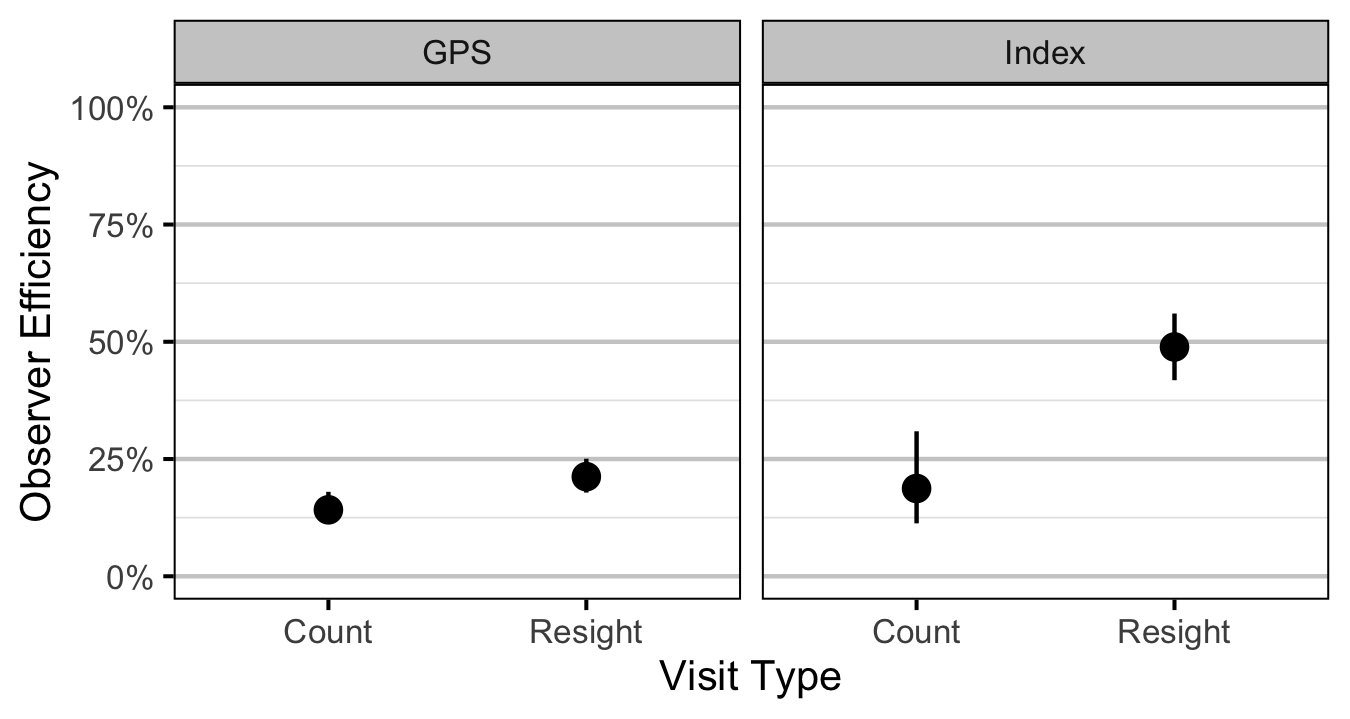
Figure 5. Predicted observer efficiency for age-1 Rainbow Trout by visit type and study design (with 95% CRIs).
Age-2
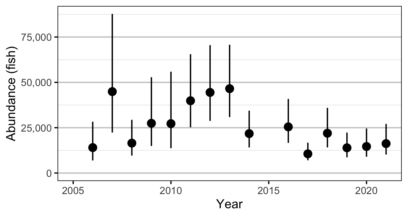
Figure 6. Predicted abundance of age-2 Rainbow Trout in the Duncan and Lardeau Rivers by year (with 95% CRIs).
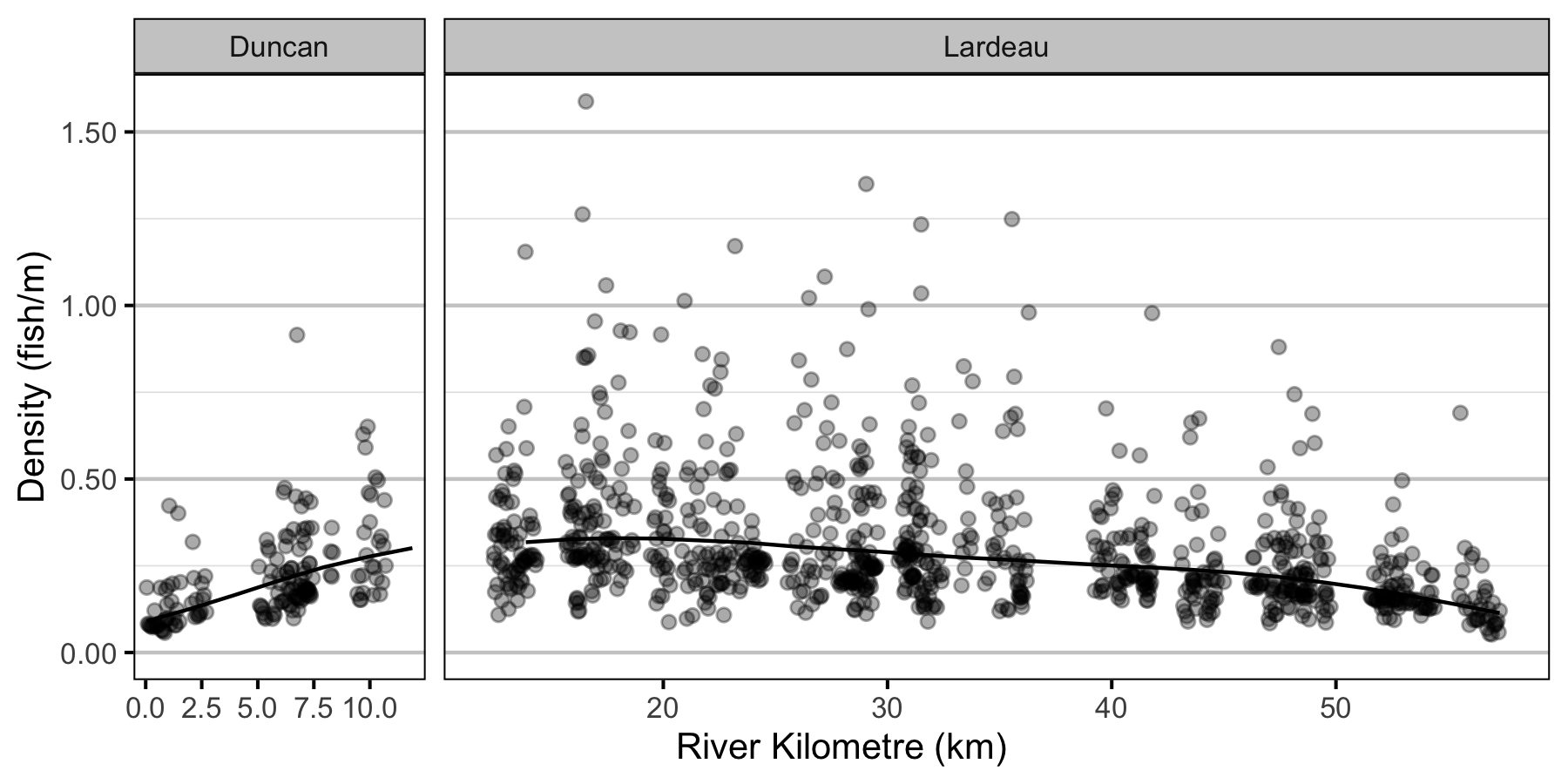
Figure 7. Predicted lineal density of age-2 Rainbow Trout in 2010 by river kilometre (with 95% CRIs).
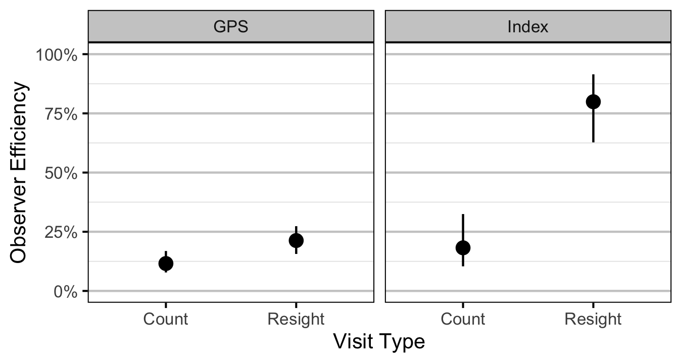
Figure 8. Predicted observer efficiency for age-2 Rainbow Trout by visit type and study design (with 95% CRIs).
Condition
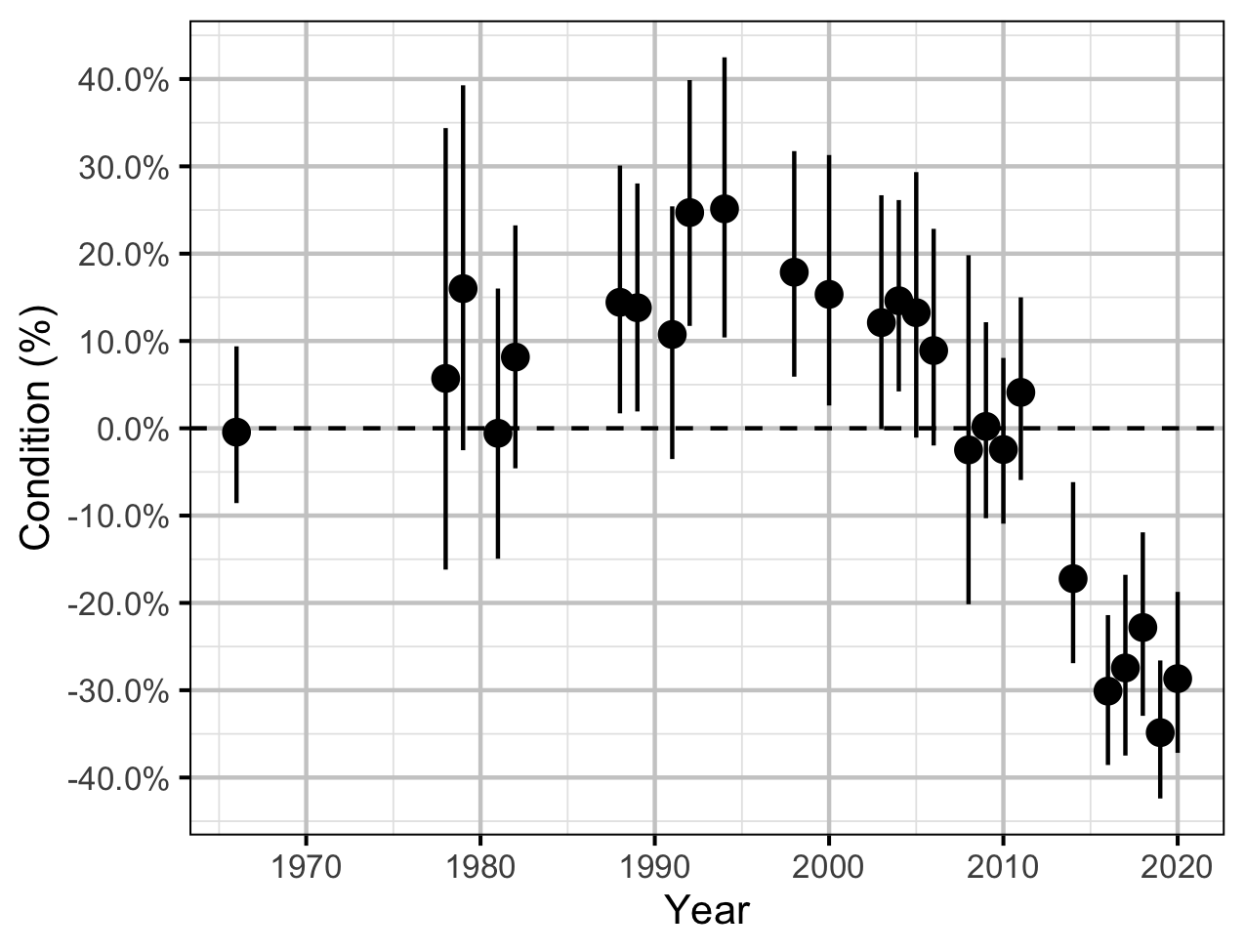
Figure 9. The percent change in the body condition for an average length fish relative to a typical year by year (with 95% CRIs).
Fecundity
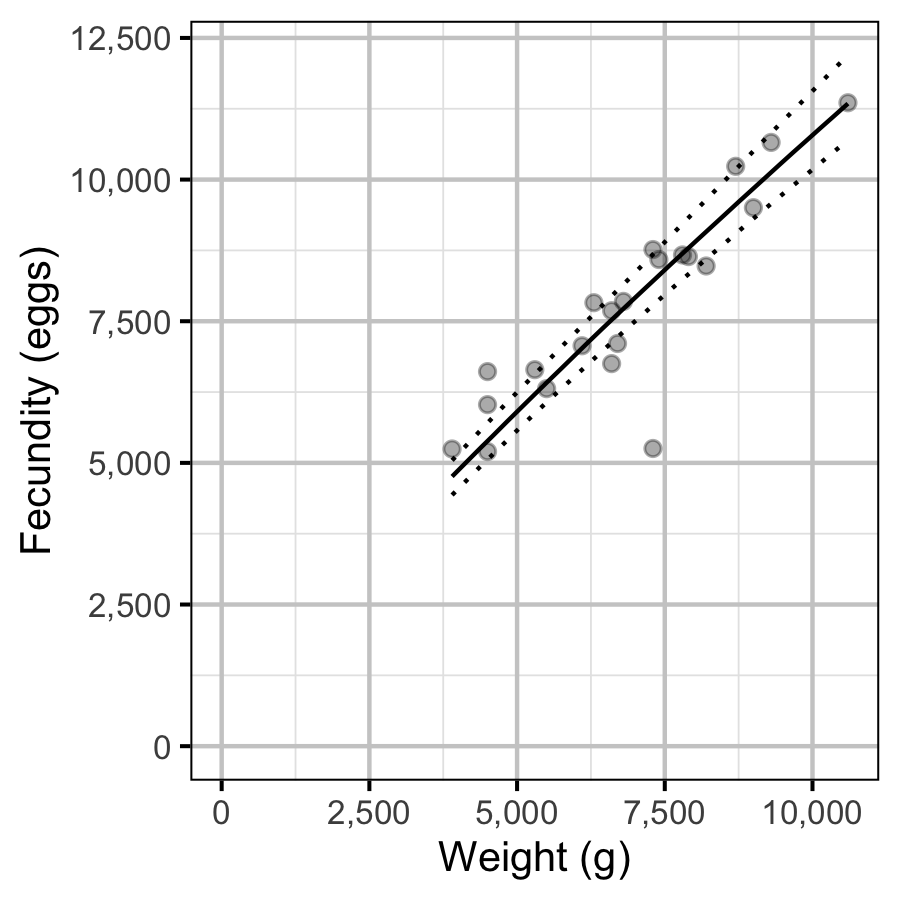
Figure 10. The fecundity-weight relationship (with 95% CRIs).
Spawner Size
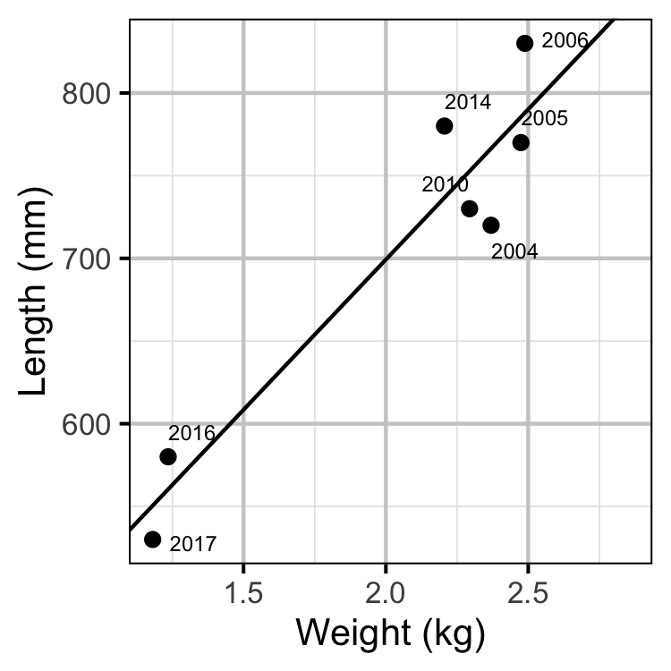
Figure 11. The mean length of spawning Rainbow Trout by the mean weight of Rainbow Trout in the KLRT.
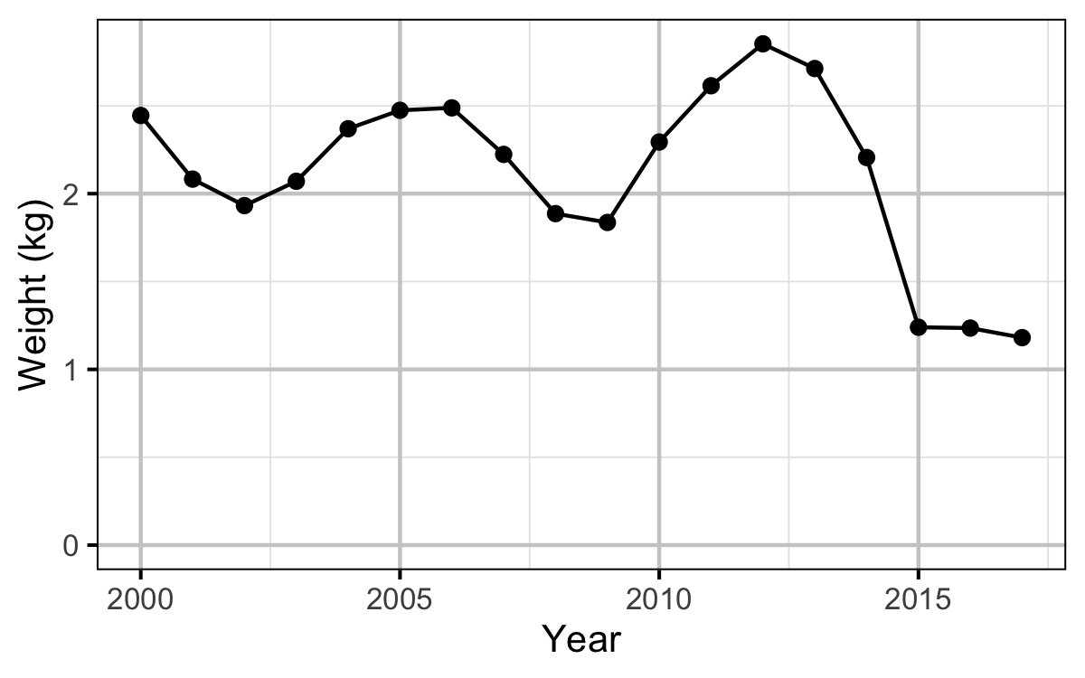
Figure 12. The mean weight of Rainbow Trout in the KLRT by year.
Egg Deposition
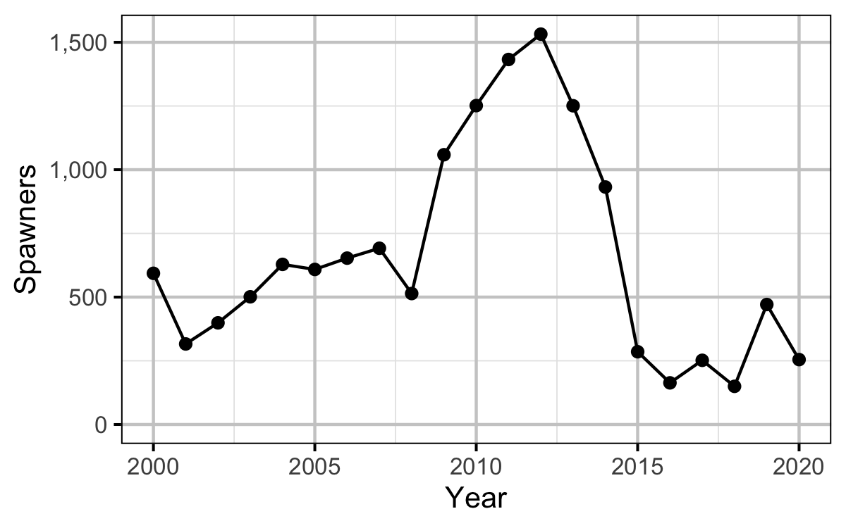
Figure 13. The spawner abundance by year.
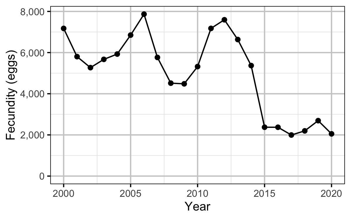
Figure 14. The estimated spawner fecundity by year.
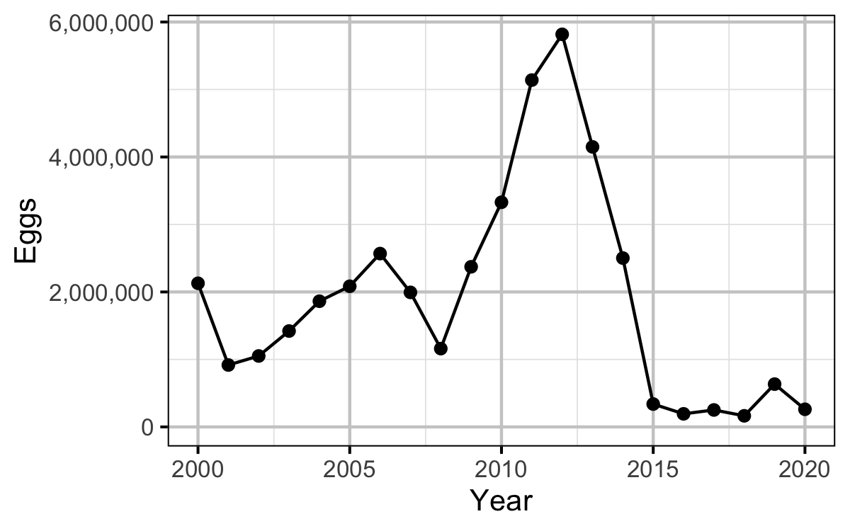
Figure 15. The egg deposition by year.
Stock-Recruitment
Age-1
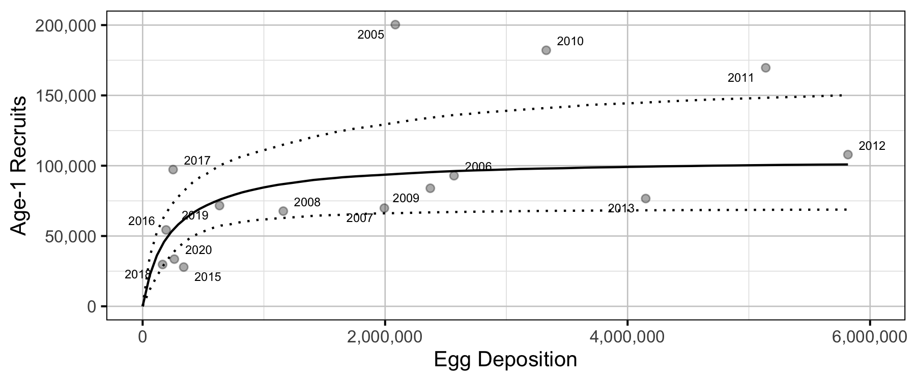
Figure 16. Predicted stock-recruitment relationship between spawners and age-1 recruits (with 95% CRIs).
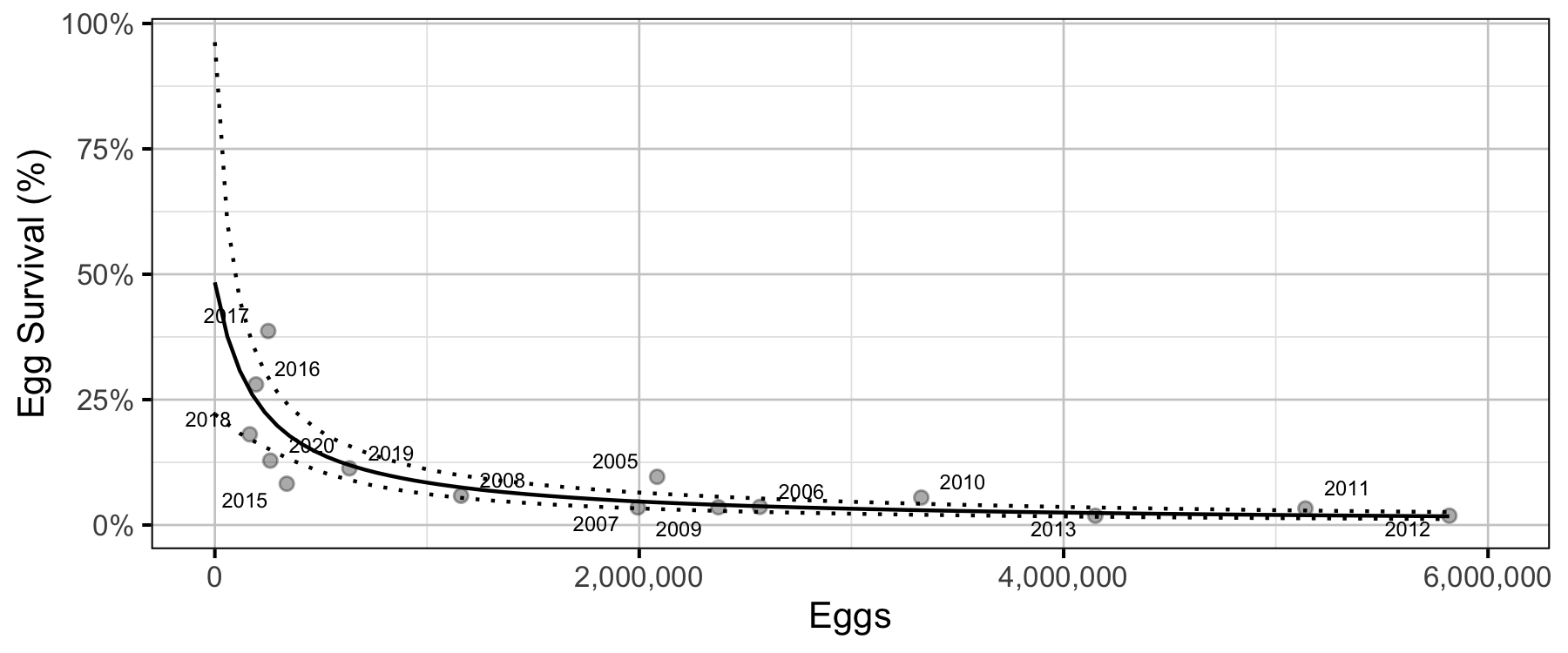
Figure 17. Predicted egg survival to age-1 by egg deposition (with 95% CRIs).
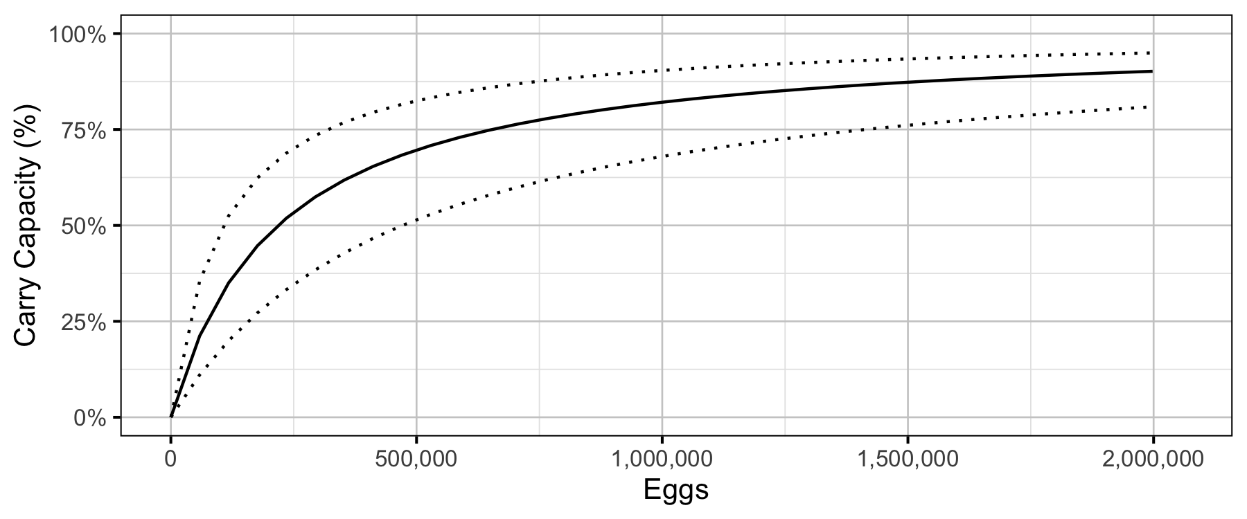
Figure 18. Predicted percent of age-1 recruits carry capacity by egg deposition (with 80% CRIs).
Age-1 to Age-2 Survival
Age-2
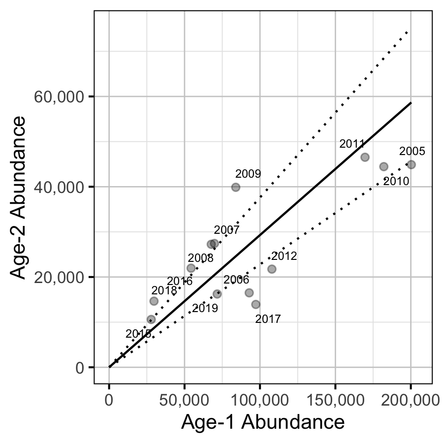
Figure 19. Predicted relationship between age-1 and age-2 abundance (with 95% CRIs).
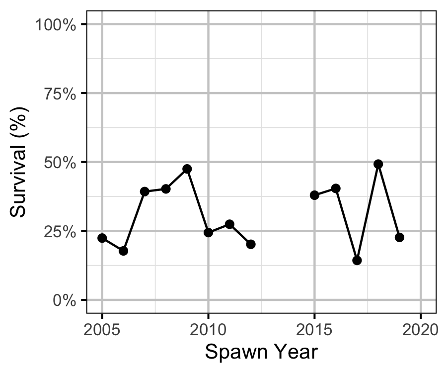
Figure 20. Estimated age-1 and age-2 survival by spawn year.
Inlake
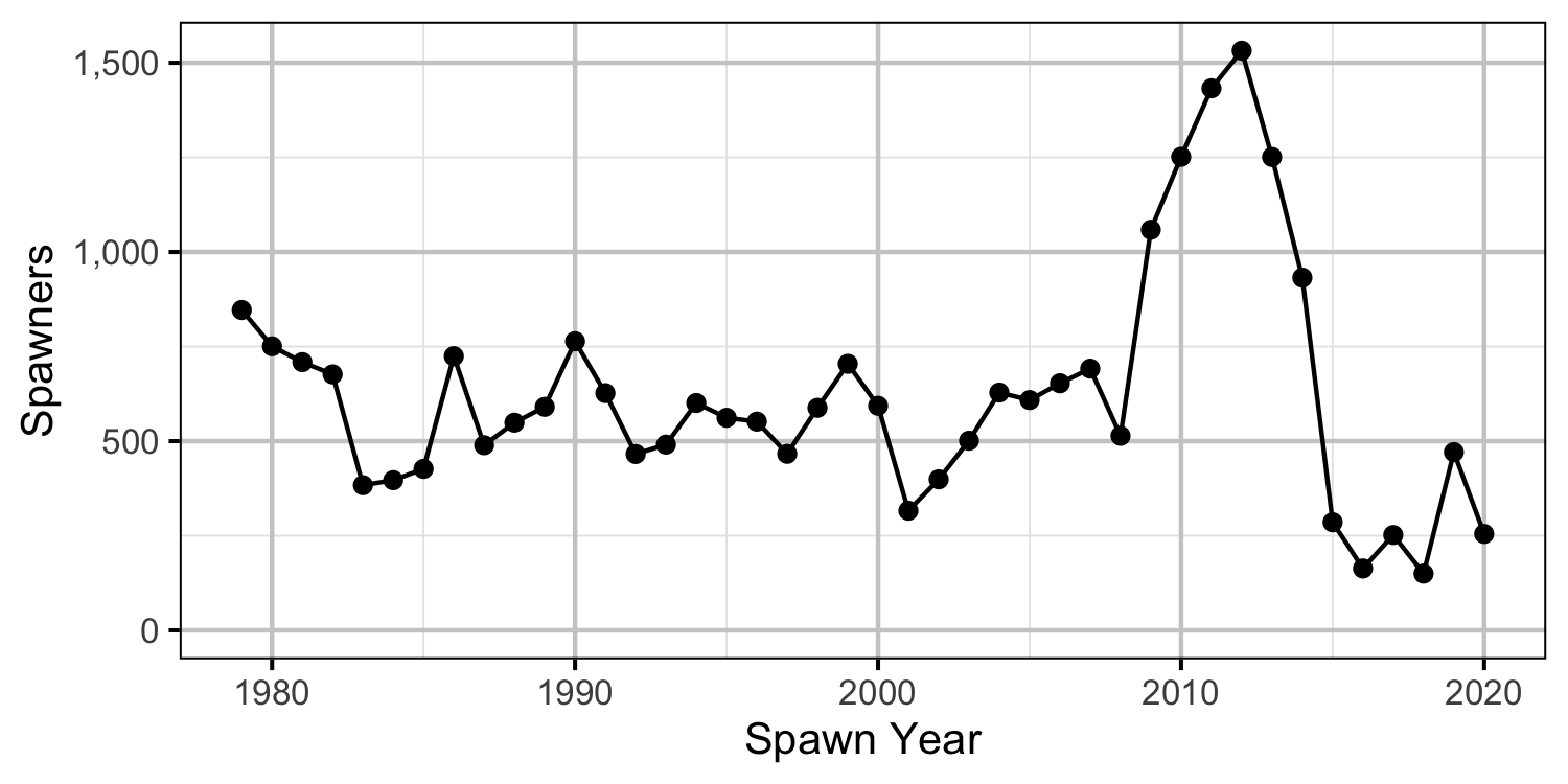
Figure 21. The number of spawners by return year.
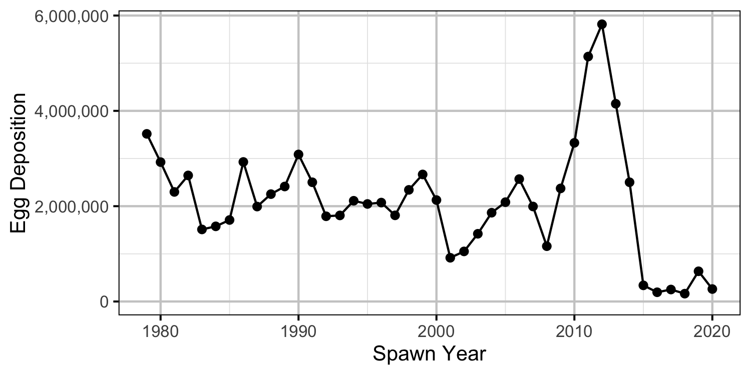
Figure 22. The estimated egg deposition by return year.
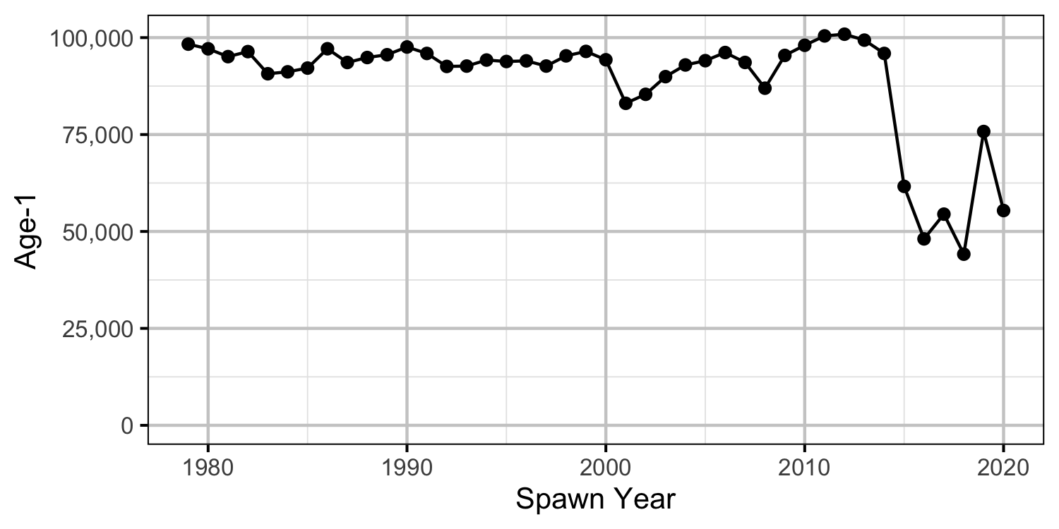
Figure 23. The number of expected age-1 recruits by spawn year based on the estimated egg deposition.
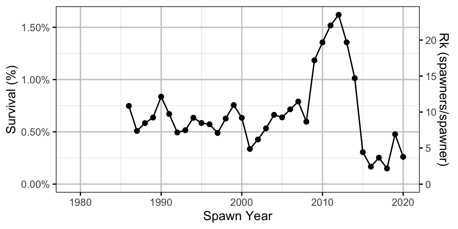
Figure 24. Survival from expected age-1 to spawners by return year.
Reproductive Rate (age-1)
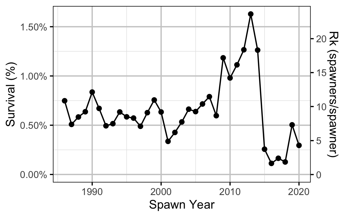
Figure 25. Survival from age-1 to spawning by return year.
Reproductive Rate (age-2)
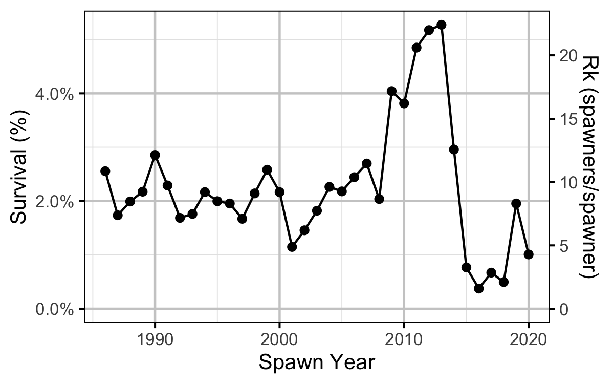
Figure 26. Survival from age-2 to spawning by return year.
Expected Spawners
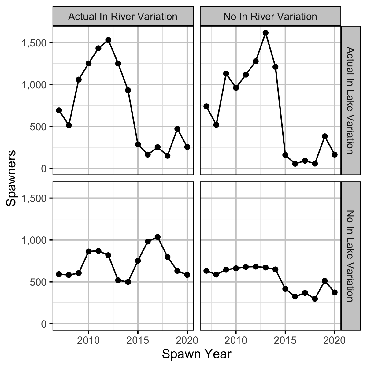
Figure 27. Expected spawners by return year and in river and in lake variation based on age-1 recruitment.
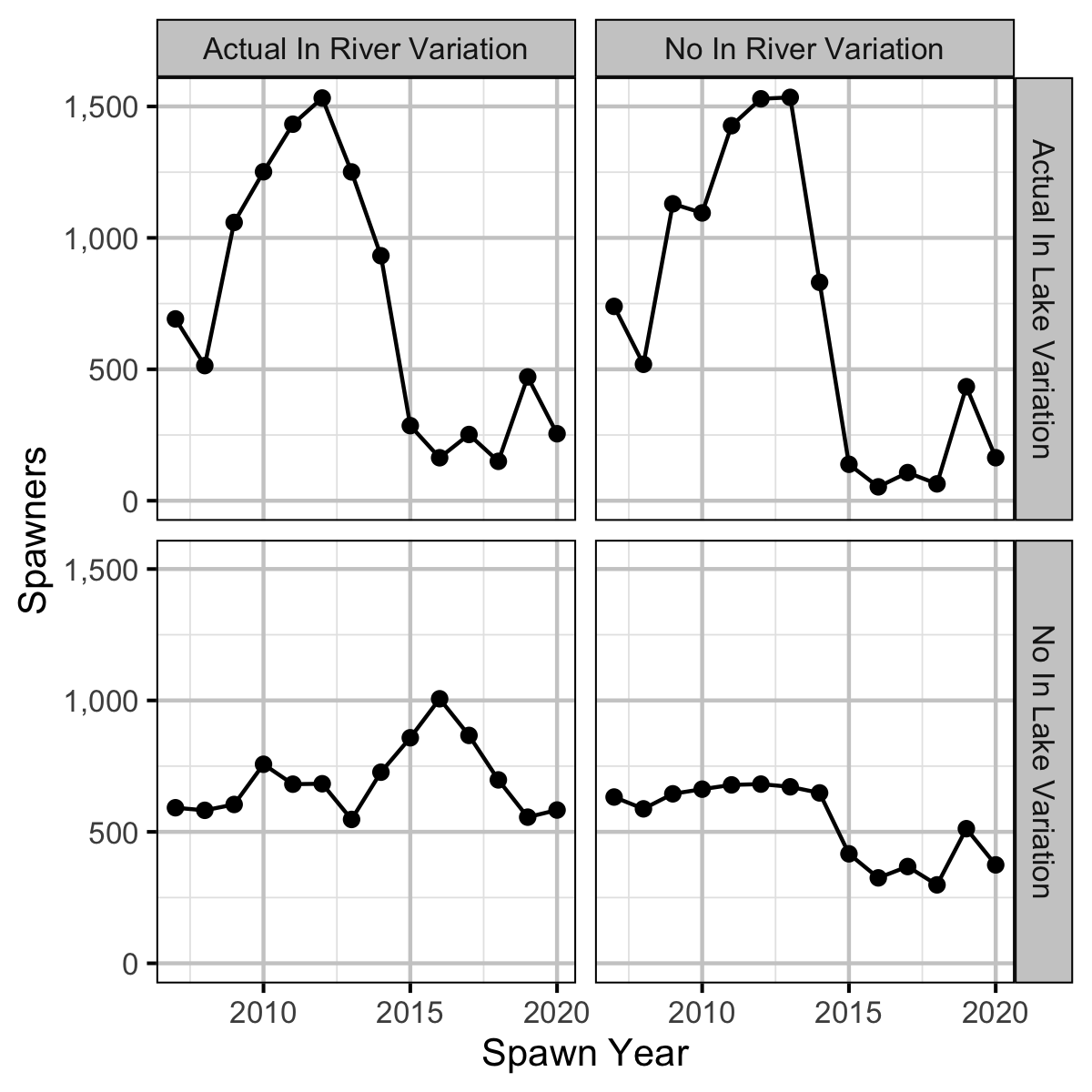
Figure 28. Expected spawners by return year and in river and in lake variation based on age-2 recruitment.
Acknowledgements
The organisations and individuals whose contributions have made this analysis report possible include:
- Habitat Conservation Trust Foundation (HCTF) and the anglers, hunters, trappers and guides who contribute to the Trust.
- Fish and Wildlife Compensation Program (FWCP) and its program partners BC Hydro, the Province of BC and Fisheries and Oceans Canada.
- Ministry of Forests, Lands and Natural Resource
Operations (MFLNRO)
- Greg Andrusak
- Matt Neufeld
- Jeff Burrows
- Tyler Weir
- Rob Bison
- Poisson Consulting
- Evan Amies-Galonski
- Seb Dalgarno
- Robyn Irvine
- Stefan Himmer
- Vicky Lipinski
- John Hagen
- Scott Decker
- Jody Schick
- Gillian Sanders
- Jeremy Baxter
- Jeff Berdusco
- Dave Derosa