Kootenay Lake Large Piscivorous Trout Hydroacoustic Analysis 2013
The suggested citation for this analytic report is:
Thorley J.L. and Hogan P.M. (2014) Kootenay Lake Large Piscivorous Trout Hydroacoustic Analysis 2013. A Poisson Consulting Analysis Report. URL: https://www.poissonconsulting.ca/f/76712537.
Background
Hierarchical Bayesian models were fitted to the hydroacoustic density data and acoustic tag depth detection for Kootenay Lake using using R version 3.0.2 (Team, 2013 ) and JAGS 3.3.0 (Plummer, 2012 ) which interfaced with each other via the jaggernaut (Thorley, 2014 ) R package. For additional information on hierarchical Bayesian modelling in the BUGS language, of which JAGS uses a dialect, the reader is referred to Kery and Schuab (2011) pages 41-44.
The hydroacoustic data was provided by the Ministry of Forest, Lands and Natural Resource Operations (MFLNRO) and the acoustic tag depth data by the Kootenay Lake Exploitation Study (Andrusak and Thorley, 2013 ).
Methods
Unless specified, the models assumed vague (low information) prior distributions (Kery and Schaub, 2011 , p. 36). The posterior distributions were estimated from a minimum of 1,000 Markov Chain Monte Carlo (MCMC) samples thinned from the second halves of three chains (Kery and Schaub, 2011 , pp. 38-40). Model convergence was confirmed by ensuring that Rhat (Kery and Schaub, 2011 , p. 40) was less than 1.1 for each of the parameters in the model (Kery and Schaub, 2011 , p. 61).
The posterior distributions of the fixed (Kery and Schaub 2011 p. 75) parameters are summarised below in terms of a point estimate (mean), lower and upper 95% credibility limits (2.5th and 97.5th percentiles), the standard deviation (SD), percent relative error (half the 95% credibility interval as a percent of the point estimate) and significance (Kery and Schaub, 2011 , p. 37,42).
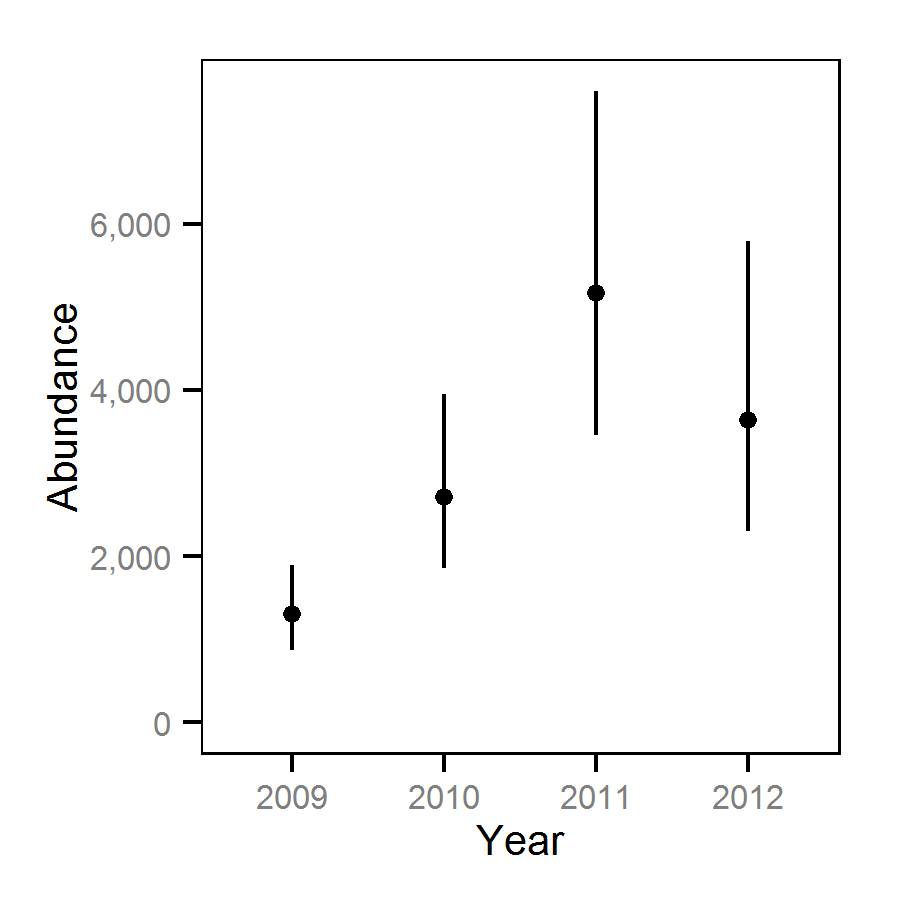
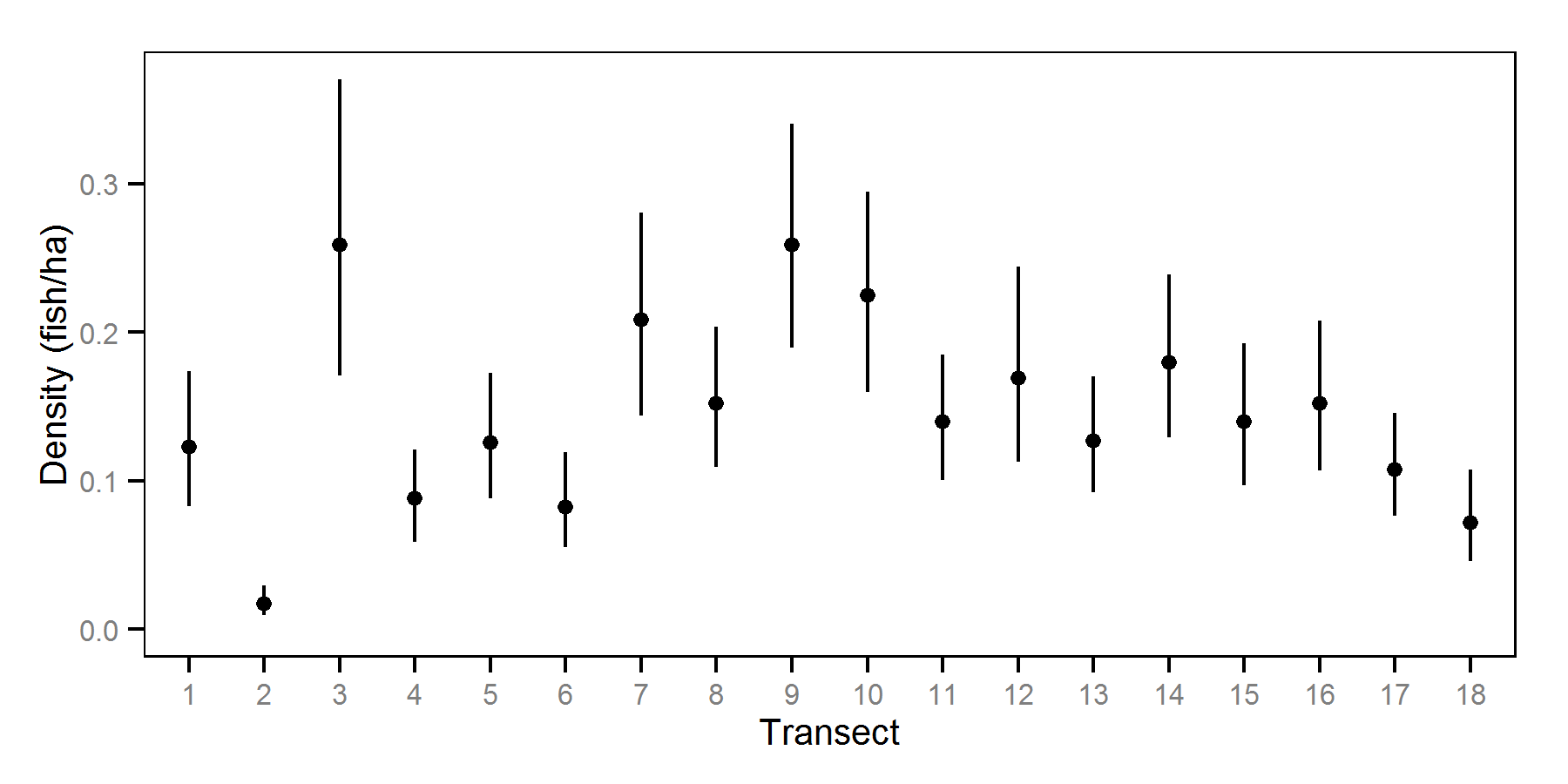
The results are displayed graphically by plotting the modeled relationships between particular variables and the response (with 95% credible intervals) with the remaining variables held constant. In general, continuous and discrete fixed variables are held constant at their mean and first level values respectively while random variables are held constant at their typical values (expected values of the underlying hyperdistributions) (Kery and Schaub, 2011 , pp. 77-82). Where informative the influence of particular variables is expressed in terms of the effect size (i.e., percent change in the response variable) with 95% credible intervals (Bradford et al. 2005 ). Plots were produced using the ggplot2 R package (Wickham, 2009 ).
Hydroacoustic Surveys
The hydroacoustic survey data were analysed using a hierarchical Bayesian zero-inflated (Kery and Schaub, 2011 , pp. 401-402) log-normal polynomial model.
Key assumptions of the hydroacoustic model include: - Positive densities (one or more fish detected) vary with year. - Positive densities vary randomly with respect to transect. - Zero-inflation varies as a third order polynomial of the standardized depth. - Density is zero-inflated log-normally distributed.
Only detections in less than 50 m of water were included in the model. The surveys were conducted during the hours of darkness. The data consisted of detection densities by decibel cutoff from 18 transects spanning 4 years.
Model Code
The JAGS model code, which uses a series of naming conventions, is presented below.
Hydroacoustic Surveys
| Variable/Parameter | Description |
|---|---|
bDepth |
Linear effect of Depth on logit(eSuitability) |
bDepth2 |
Quadratic effect of Depth on logit(eSuitability) |
bDepth3 |
Cubic effect of Depth on logit(eSuitability) |
bIntercept |
Intercept of eLogDensity |
bSuitable |
Intercept of logit(eSuitability) |
bTransect[tr] |
Linear effect of trth transect on eLogDensity |
bYear[yr] |
Linear effect of yrth year on eLogDensity |
Density[i] |
Observed density on ith transect depth survey |
Depth[i] |
Standardised depth of ith transect depth survey |
eLogDensity[i] |
Expected log density on ith transect depth survey |
eSuitability[i] |
Expected probability of positive density on ith transect depth survey |
sDensity |
SD of the residual log-normal density |
sTransect |
SD of bTransect |
Hydroacoustic Surveys - Model 1
model {
  bIntercept ~ dnorm(0, 2^-2)
  bSuitable ~ dnorm(0, 2^-2)

  sDensity ~ dunif(0, 2)

  bYear[1] <- 0
  for(yr in 2:nYear) {
    bYear[yr] ~ dnorm(0, 2^-2)
  }

  bDepth ~ dnorm(0, 2^-2)
  bDepth2 ~ dnorm(0, 2^-2)
  bDepth3 ~ dnorm(0, 2^-2)

  sTransect ~ dunif(0, 2)
  for(tr in 1:nTransect) {
    bTransect[tr] ~ dnorm(0, sTransect^-2)
  }

  for (i in 1:length(Depth)) {
    eLogDensity[i] <- bIntercept + bYear[Year[i]]  + bTransect[Transect[i]]
    logit(eSuitable[i]) <- bSuitable + bDepth * Depth[i]
      + bDepth2 * Depth[i]^2 + bDepth3 * Depth[i]^3

    dFish[i] ~ dbern(eSuitable[i])
    dLogDensity[i] <- ifelse(dFish[i], eLogDensity[i], log(0.00001))
    Density[i] ~ dlnorm(dLogDensity[i], sDensity^-2)
  }
}
Parameter Estimates
The posterior distributions for the fixed (Kery and Schaub 2011 p. 75) parameters in each model are summarised below.
Hydroacoustic Surveys - July - -33 Decibels
| Parameter | Estimate | Lower | Upper | SD | Error | Significance |
|---|---|---|---|---|---|---|
| bDepth | -1.8033 | -2.52230 | -1.0699 | 0.370650 | 40 | 0.0000 |
| bDepth2 | -2.1369 | -2.81402 | -1.5521 | 0.323180 | 30 | 0.0000 |
| bDepth3 | 0.7775 | 0.03492 | 1.4304 | 0.344780 | 90 | 0.0379 |
| bIntercept | -0.7290 | -1.09462 | -0.3612 | 0.182280 | 50 | 0.0000 |
| bSuitable | -0.9951 | -1.34131 | -0.7030 | 0.164530 | 32 | 0.0000 |
| bYear[2] | 0.7341 | 0.58320 | 0.8828 | 0.077983 | 20 | 0.0000 |
| bYear[3] | 1.3768 | 1.23617 | 1.5233 | 0.075969 | 10 | 0.0000 |
| bYear[4] | 1.0164 | 0.73771 | 1.3046 | 0.148530 | 28 | 0.0000 |
| sDensity | 0.2331 | 0.22256 | 0.2448 | 0.005738 | 5 | 0.0000 |
| sTransect | 0.6931 | 0.46332 | 1.0175 | 0.145530 | 40 | 0.0000 |
Hydroacoustic Surveys - July - -32 Decibels
| Parameter | Estimate | Lower | Upper | SD | Error | Significance |
|---|---|---|---|---|---|---|
| bDepth | -2.01608 | -3.37031 | -0.75880 | 0.660740 | 65 | 0.0000 |
| bDepth2 | -1.66246 | -2.98013 | -0.72550 | 0.553370 | 68 | 0.0000 |
| bDepth3 | 0.51071 | -0.57459 | 1.45855 | 0.520380 | 199 | 0.3072 |
| bIntercept | -0.31265 | -0.84010 | 0.26592 | 0.308940 | 177 | 0.3498 |
| bSuitable | -2.84400 | -3.51732 | -2.28938 | 0.307000 | 22 | 0.0000 |
| bYear[2] | 0.58501 | 0.47008 | 0.70451 | 0.059740 | 20 | 0.0000 |
| bYear[3] | 0.54197 | 0.42181 | 0.66805 | 0.061617 | 23 | 0.0000 |
| bYear[4] | 0.55857 | 0.31891 | 0.79469 | 0.118180 | 43 | 0.0000 |
| sDensity | 0.08402 | 0.08007 | 0.08839 | 0.002148 | 5 | 0.0000 |
| sTransect | 0.96926 | 0.60838 | 1.56124 | 0.239070 | 49 | 0.0000 |
Hydroacoustic Surveys - September - -33 Decibels
| Parameter | Estimate | Lower | Upper | SD | Error | Significance |
|---|---|---|---|---|---|---|
| bDepth | 0.53101 | -0.2222 | 1.3505 | 0.410850 | 148 | 0.1936 |
| bDepth2 | -3.44685 | -4.3541 | -2.6280 | 0.439780 | 25 | 0.0000 |
| bDepth3 | -0.63124 | -1.7505 | 0.4658 | 0.574580 | 176 | 0.2874 |
| bIntercept | -0.60551 | -0.8043 | -0.4124 | 0.101940 | 32 | 0.0000 |
| bSuitable | -0.48413 | -0.7801 | -0.1949 | 0.147290 | 60 | 0.0060 |
| bYear[2] | 0.08771 | -0.0595 | 0.2243 | 0.069976 | 162 | 0.2116 |
| bYear[3] | 1.51410 | 1.3505 | 1.6640 | 0.081539 | 10 | 0.0000 |
| bYear[4] | 0.59134 | 0.3473 | 0.8333 | 0.124540 | 41 | 0.0000 |
| sDensity | 0.24535 | 0.2341 | 0.2580 | 0.006253 | 5 | 0.0000 |
| sTransect | 0.36754 | 0.2404 | 0.5499 | 0.077297 | 42 | 0.0000 |
Hydroacoustic Surveys - September - -32 Decibels
| Parameter | Estimate | Lower | Upper | SD | Error | Significance |
|---|---|---|---|---|---|---|
| bDepth | -0.43852 | -1.60497 | 0.61084 | 0.565930 | 253 | 0.4290 |
| bDepth2 | -3.81101 | -5.38164 | -2.49603 | 0.743030 | 38 | 0.0000 |
| bDepth3 | -0.53423 | -2.12642 | 1.09748 | 0.831900 | 302 | 0.4908 |
| bIntercept | -0.09416 | -0.35094 | 0.16003 | 0.125920 | 271 | 0.4309 |
| bSuitable | -1.42946 | -1.84198 | -1.06056 | 0.200880 | 27 | 0.0000 |
| bYear[2] | -0.69404 | -0.76953 | -0.61378 | 0.039188 | 11 | 0.0000 |
| bYear[3] | 0.28385 | 0.19054 | 0.37437 | 0.048683 | 32 | 0.0000 |
| bYear[4] | 0.09459 | -0.00848 | 0.20825 | 0.054347 | 115 | 0.0773 |
| sDensity | 0.07548 | 0.07191 | 0.07941 | 0.001931 | 5 | 0.0000 |
| sTransect | 0.46874 | 0.32598 | 0.68769 | 0.092371 | 39 | 0.0000 |
Figures
Hydroacoustic Surveys - July - -33 Decibels
Hydroacoustic Surveys - July - -32 Decibels
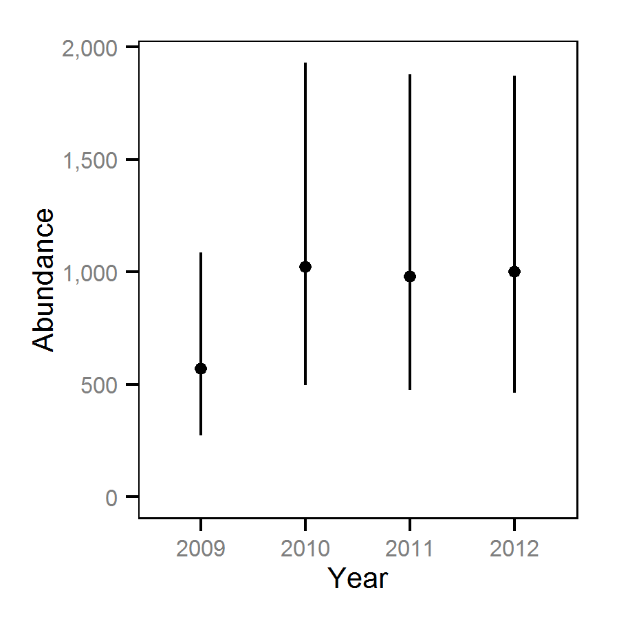
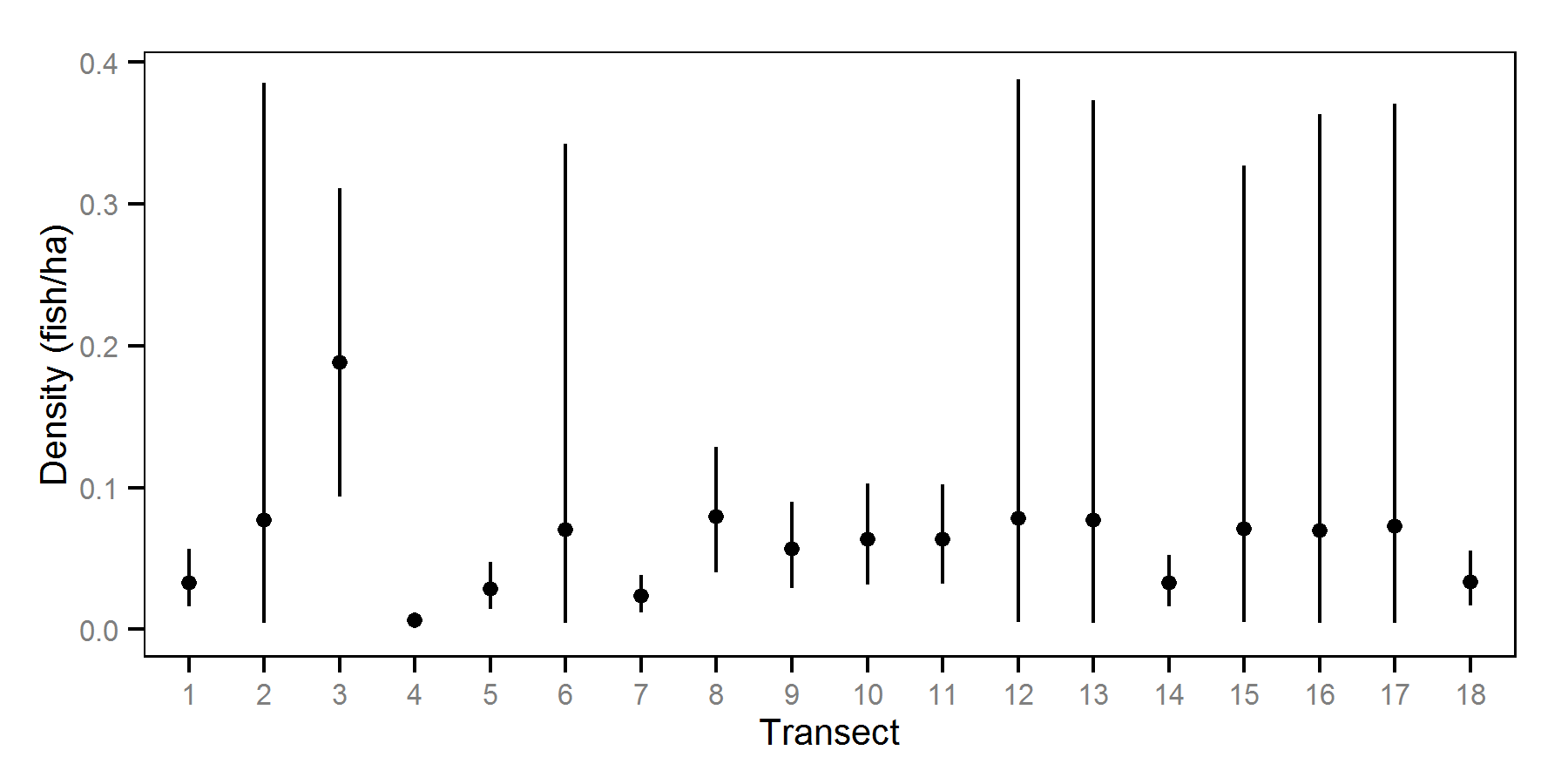
Hydroacoustic Surveys - September - -33 Decibels
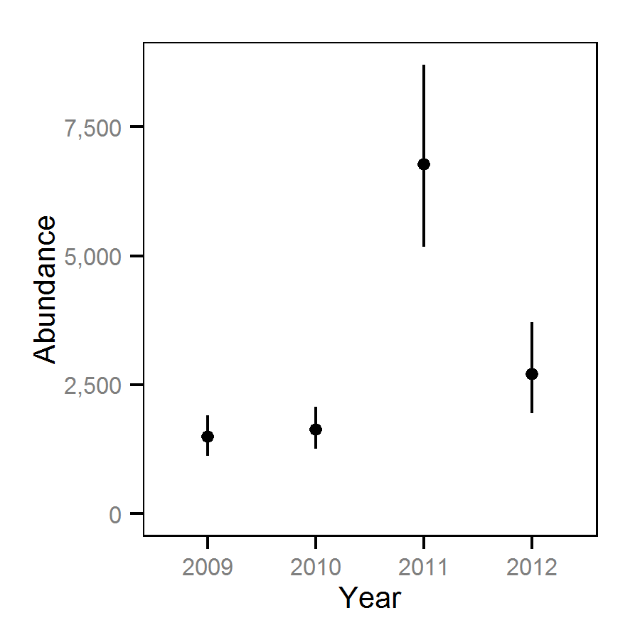
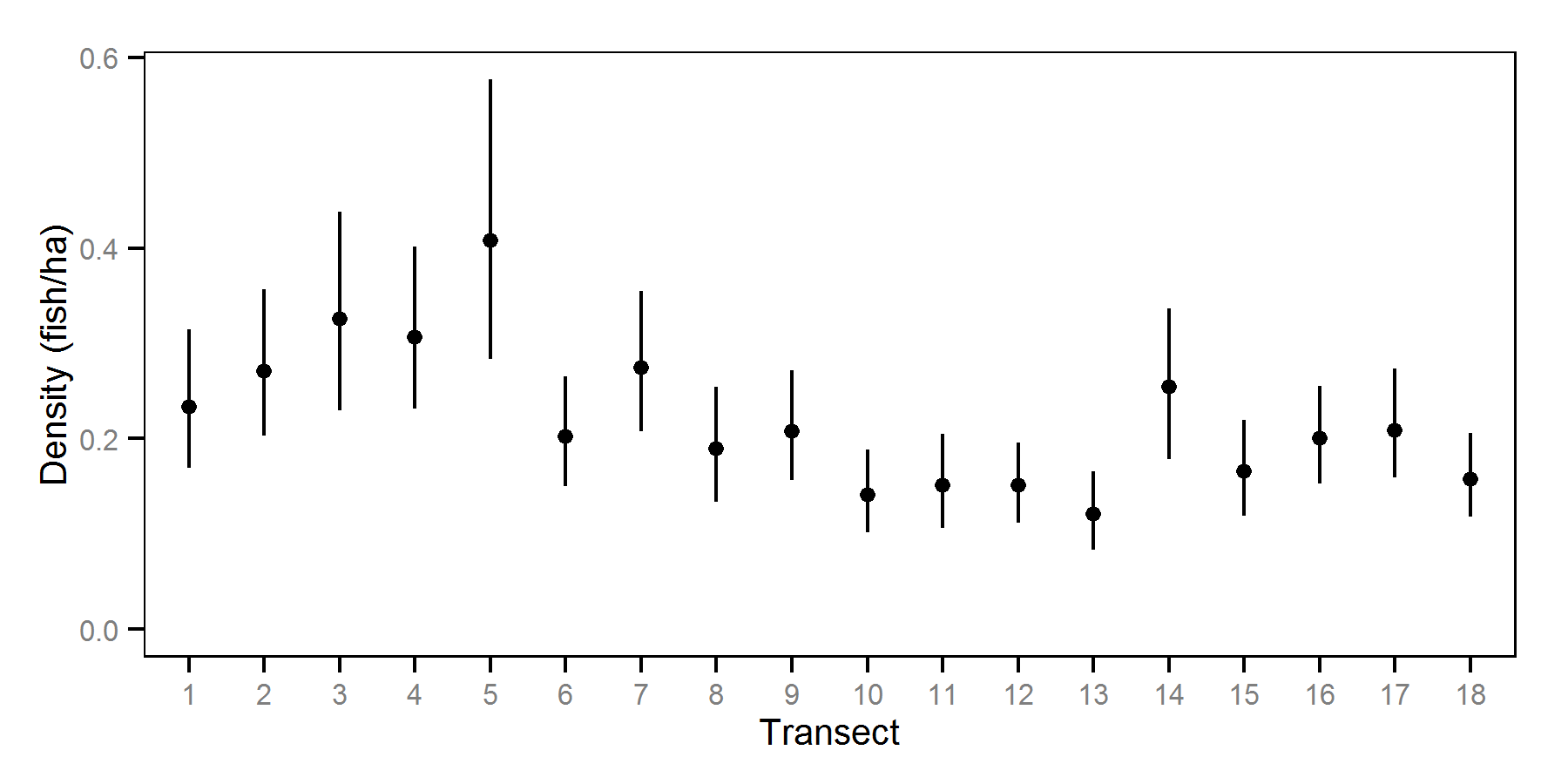
Hydroacoustic Surveys - September - -32 Decibels
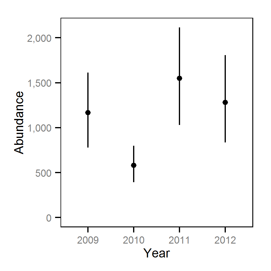
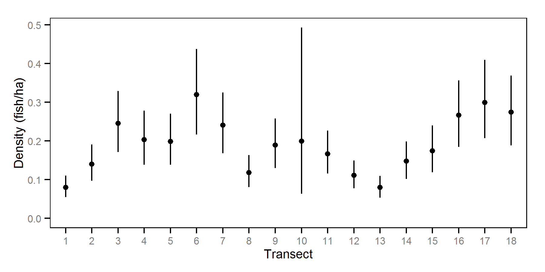
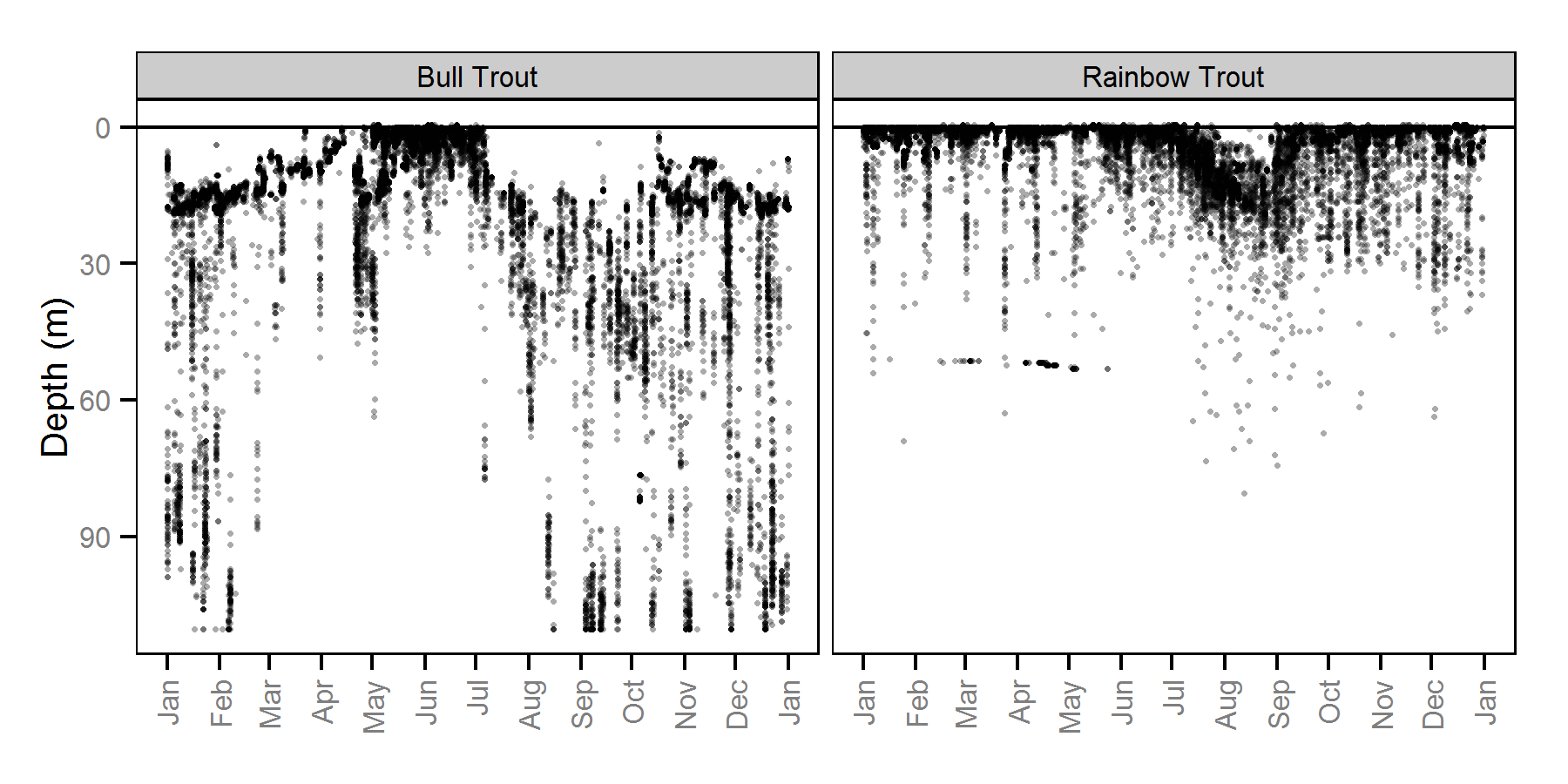
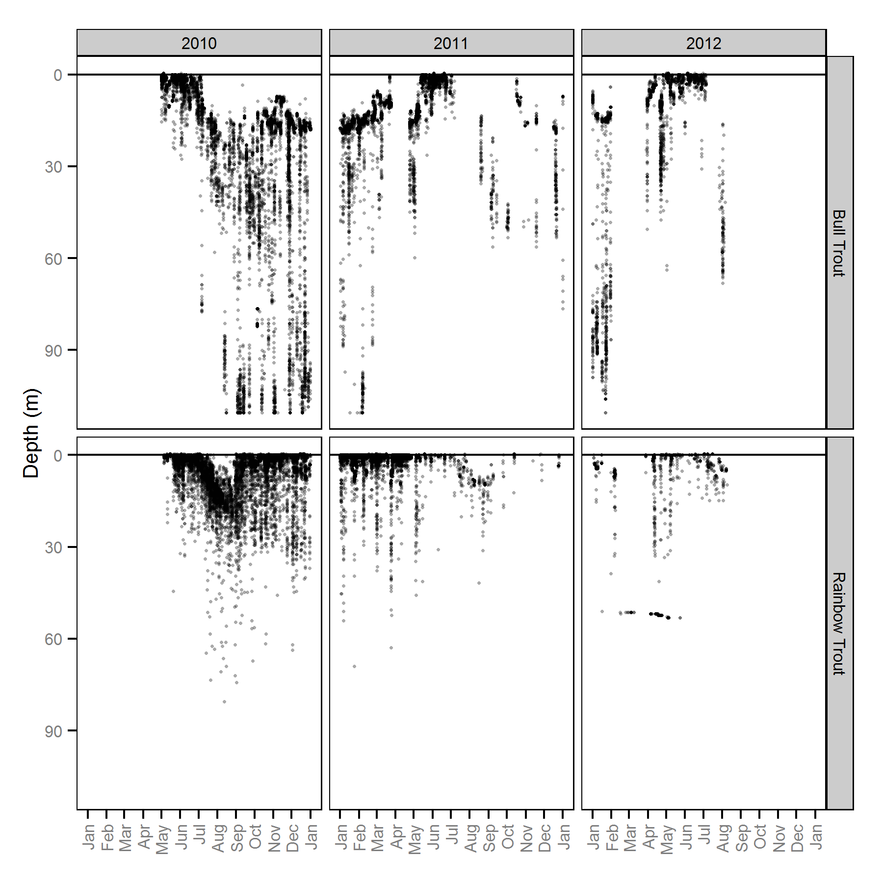
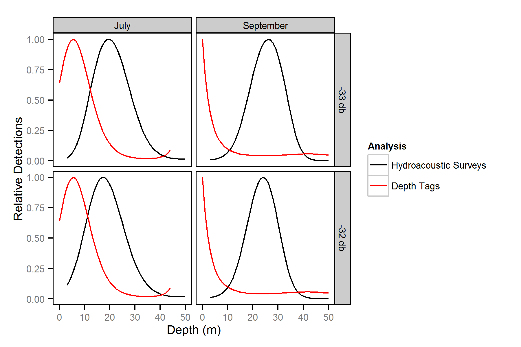
Depth Distributions
Acknowledgements
This analysis was made possible through the support of the following organisations:
- Habitat Conservation Trust Foundation (HCTF) and the anglers, hunters, trappers and guides who contribute to the Trust
- Ministry of Forests, Lands and Natural Resource Operations (MFLNRO)
- Redfish Consulting
References
- Greg Andrusak, Joseph Thorley, (2013) Kootenay Lake Exploitation Study: Fishing and Natural Mortality of Large Rainbow Trout and Bull Trout: 2013 Annual Report.
- Michael Bradford, Josh Korman, Paul Higgins, (2005) Using confidence intervals to estimate the response of salmon populations (Oncorhynchus spp.) to experimental habitat alterations. Canadian Journal of Fisheries and Aquatic Sciences 62 (12) 2716-2726 10.1139/f05-179
- Hadley Wickham, (2009) ggplot2: elegant graphics for data analysis. http://had.co.nz/ggplot2/book
- Joseph Thorley, (2014) jaggernaut: An R package to facilitate Bayesian analyses using JAGS (Just Another Gibbs Sampler). https://github.com/joethorley/jaggernaut
- Marc Kery, Michael Schaub, (2011) Bayesian population analysis using {WinBUGS} : a hierarchical perspective.
- Martyn Plummer, (2012) {JAGS} Version 3.3.0 User Manual. http://sourceforge.net/projects/mcmc-jags/files/Manuals/3.x/
- R Team, (2013) R: A Language and Environment for Statistical Computing. http://www.R-project.org
