Kootenay Lake Gerrard Rainbow Trout Condition and Growth Analysis 2014
The suggested citation for this analytic report is:
Thorley, J.L. & Andrusk, G.F. (2015) Kootenay Lake Gerrard Rainbow Trout Condition and Growth Analysis 2014. A Poisson Consulting Analysis Report. URL: https://www.poissonconsulting.ca/f/723490014.
Background
The large, piscivorous Gerrard Rainbow Trout of Kootenay Lake support an important recreational fishery. Intermittently, since 1966, length, weight, fecundity and scale information has been collected from individual fish.
The primary questions the following analyses attempt to answer are:
What is the relationship between fork length and a) weight and b) fecundity?
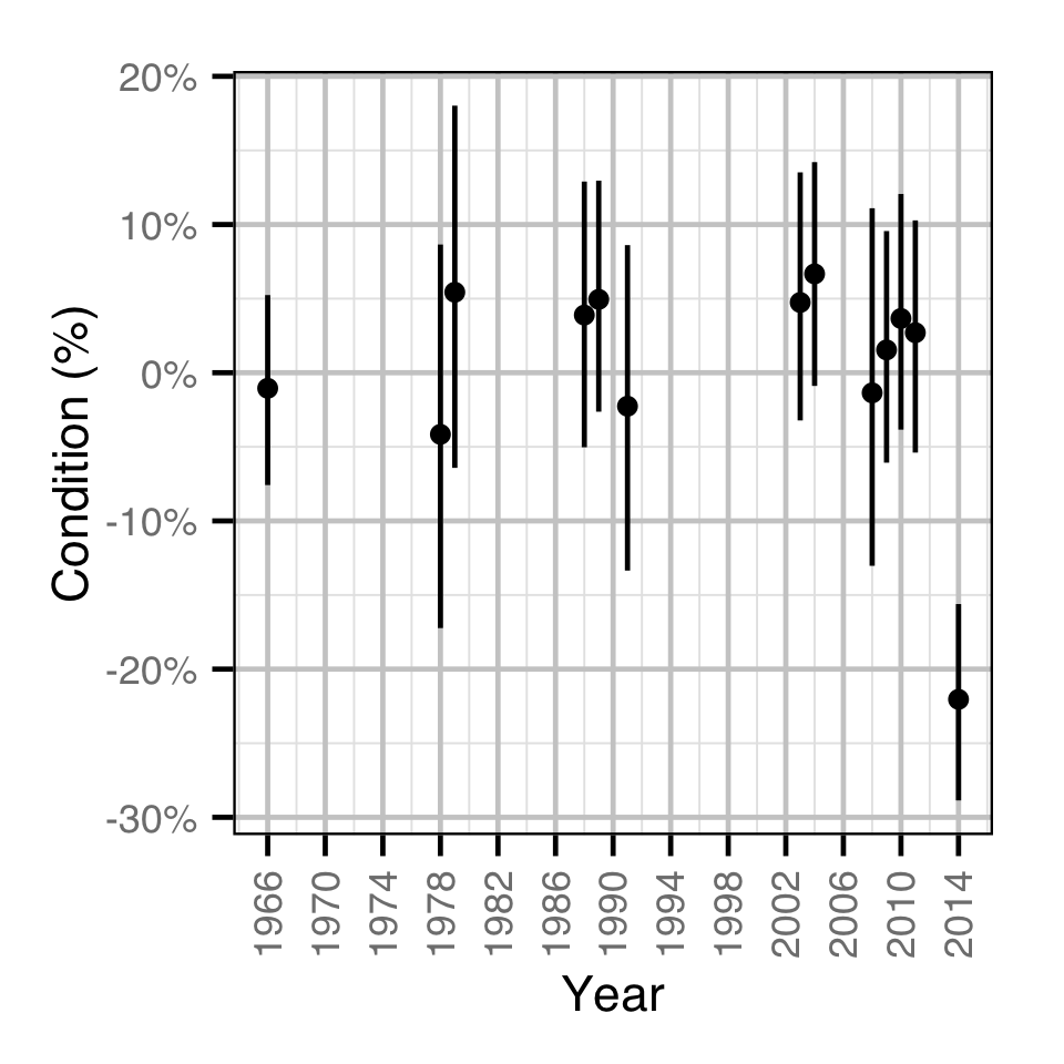
How does body condition vary by year?
How does growth vary by year?
In addition the analysis asks
Are trends in growth and condition related to trends in kokanee abundance?
Methods
Data Preparation
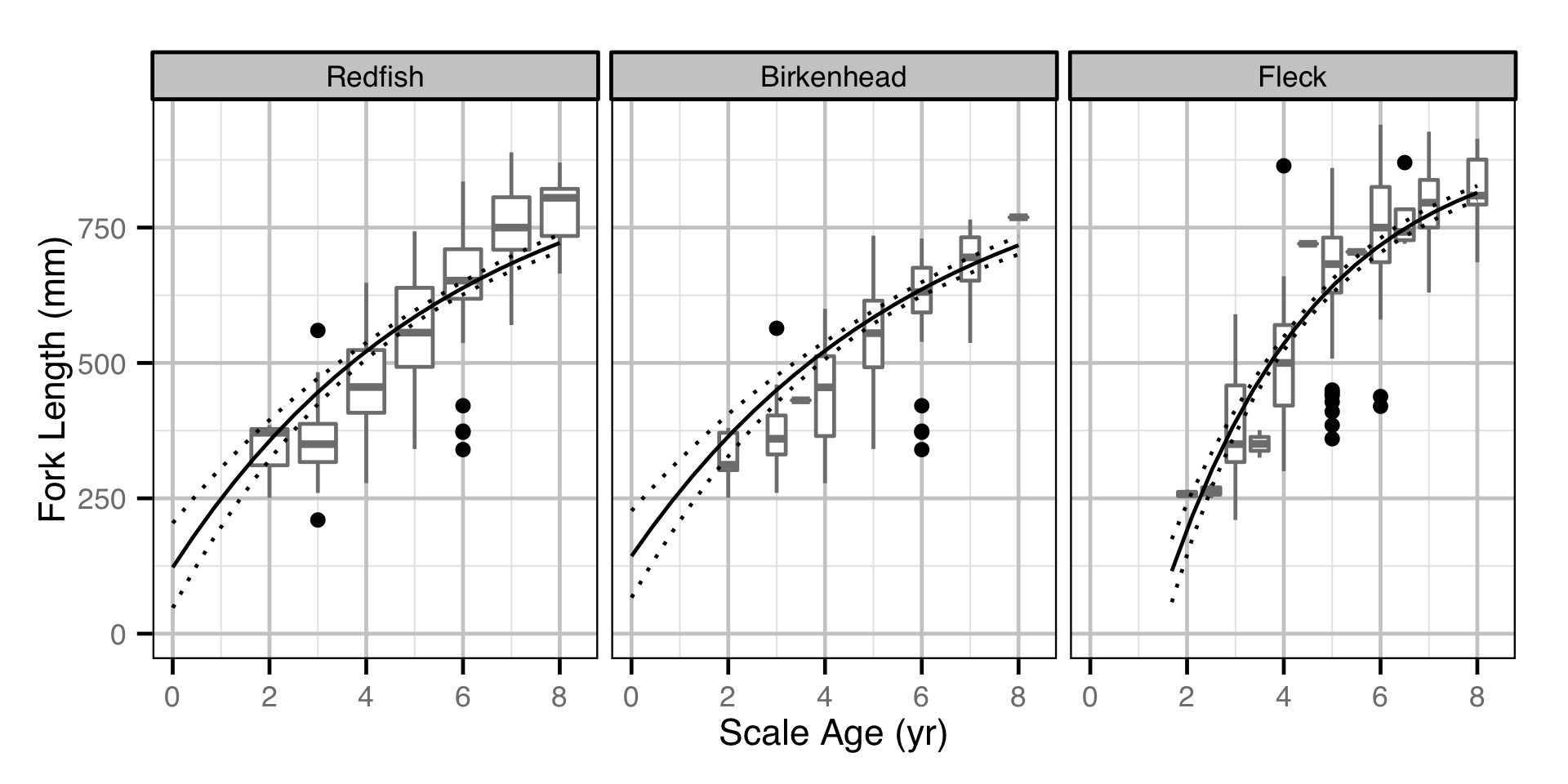
The length, weight, fecundity and kokanee information was provided by RedFish Consulting Ltd. Scale ages were determined by Greg Andrusak (RedFish Consulting Ltd.), Carol Lidstone (Birkenhead Scale Analyses) and Les Fleck. Scale radii at annuli and scale lengths were provided by Greg Andrusak. The data were cleansed, tidied and manipulated prior to analysis using R version 3.1.2 (Team 2013).
Statistical Analysis
Hierarchical Bayesian models were fitted to the count data using R version 3.1.2 (Team 2013) and JAGS 3.4.0 (Plummer 2012) which interfaced with each other via jaggernaut 2.2.8 (Thorley 2013). For additional information on hierarchical Bayesian modelling in the BUGS language, of which JAGS uses a dialect, the reader is referred to Kery and Schaub (2011, 41–44).
Unless specified, the models assumed vague (low information) prior distributions (Kery and Schaub 2011, 36). The posterior distributions were estimated from a minimum of 1,000 Markov Chain Monte Carlo (MCMC) samples thinned from the second halves of three chains (Kery and Schaub 2011, 38–40). Model convergence was confirmed by ensuring that Rhat (Kery and Schaub 2011, 40) was less than 1.1 for each of the parameters in the model (Kery and Schaub 2011, 61). Model adequacy was confirmed by examination of residual plots.
The posterior distributions of the fixed (Kery and Schaub 2011, 75) parameters are summarised in terms of a point estimate (mean), lower and upper 95% credible limits (2.5th and 97.5th percentiles), the standard deviation (SD), percent relative error (half the 95% credible interval as a percent of the point estimate) and significance (Kery and Schaub 2011, 37, 42).
Variable selection was achieved by dropping insignificant (Kery and Schaub 2011, 37, 42) fixed (Kery and Schaub 2011, 77–82) variables and uninformative random variables. A fixed variables was considered to be insignificant if its significance was \(\geq\) 0.05 while a random variable was considered to be uninformative if its percent relative error was \(\geq\) 80%.
The results are displayed graphically by plotting the modeled relationships between particular variables and the response with 95% credible intervals (CRIs) with the remaining variables held constant. In general, continuous and discrete fixed variables are held constant at their mean and first level values respectively while random variables are held constant at their typical values (expected values of the underlying hyperdistributions) (Kery and Schaub 2011, 77–82). Where informative the influence of particular variables is expressed in terms of the effect size (i.e., percent change in the response variable) with 95% CRIs (Bradford et al. 2005).
Fecundity
The relationship between fork length and the egg count was estimated using an allometric model. Key assumptions of the fecundity model include:
- The residual egg counts are log-normally distributed.
Condition
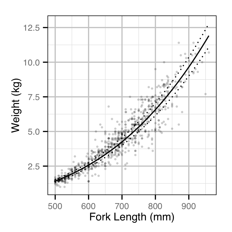
The relationship between body weight and fork length was estimated using an allometric mass-length model similar to He and Bence (2008). Key assumptions of the condition model include:
- The weight varies with the length.
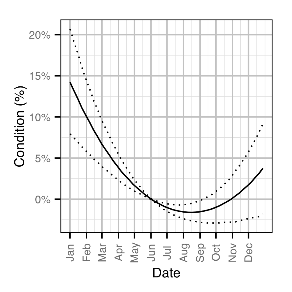
- The weight varies with the day of the year as a second order polynomial.
- The weight varies randomly with the year
- The residual weight is log-normally distributed.
Backcalculated Growth
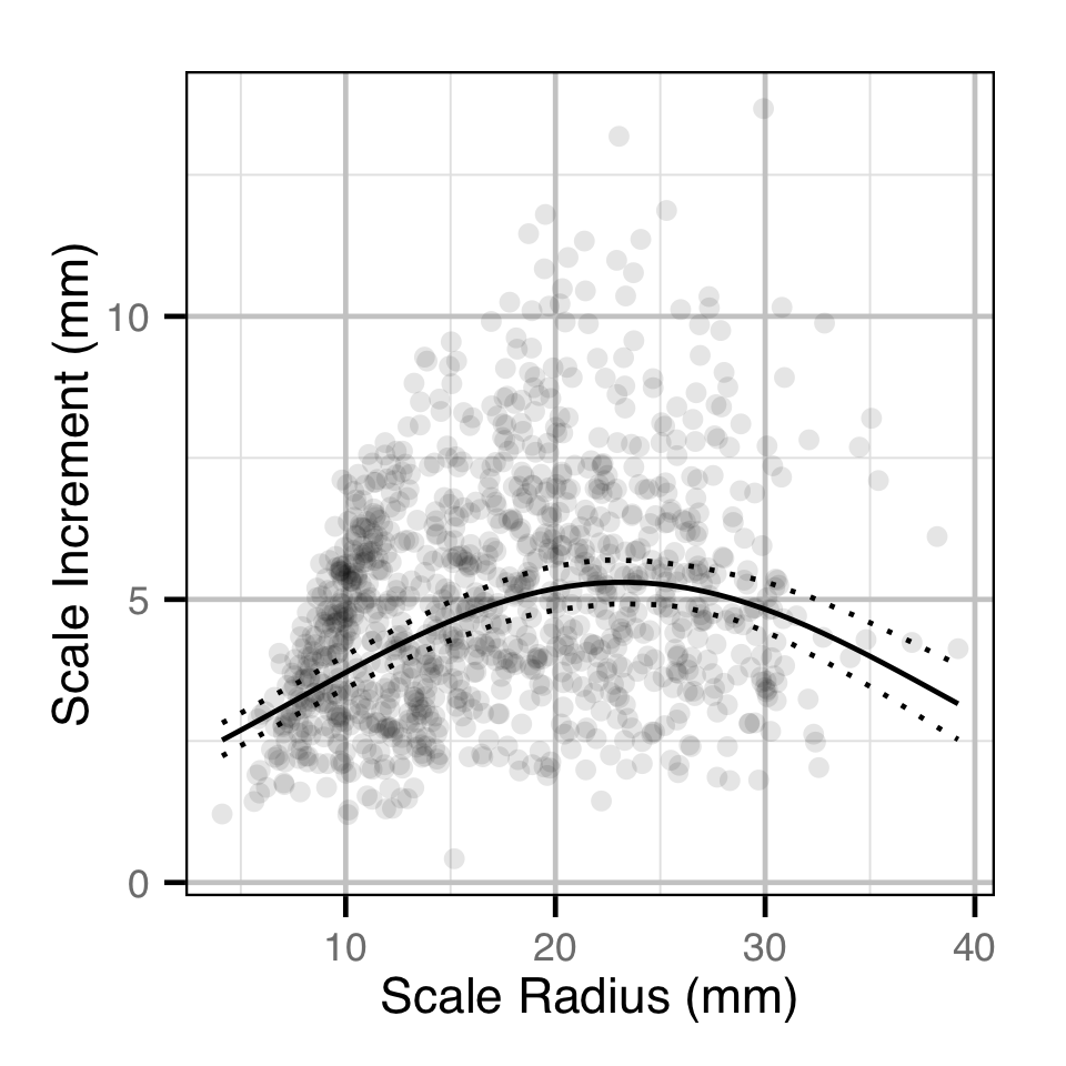
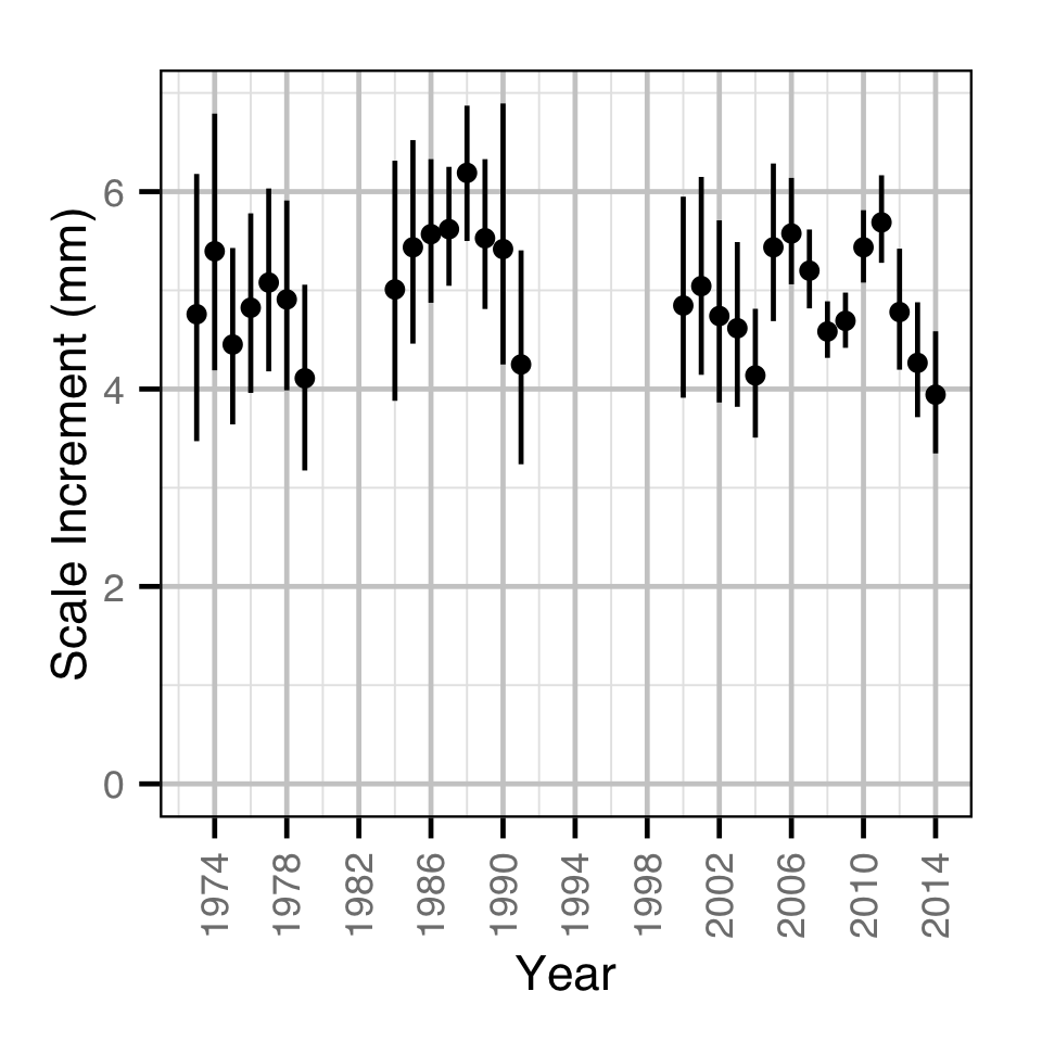
The relative growth in any given year was estimated from the scale increments using a polynomial model. Key assumptions of the polynomial model include:
- The scale increment varies with the scale radius as a second order polynomial.
- The scale increment varies randomly by year.
- The residual variation which is log-normally distributed varies with the reader’s minimum confidence in the two annuli.
Preliminary analyses indicated that the fork length of the fish at capture and fish ID as a random effect were not informative predictors of scale increment.
Dynamic Factor Analysis
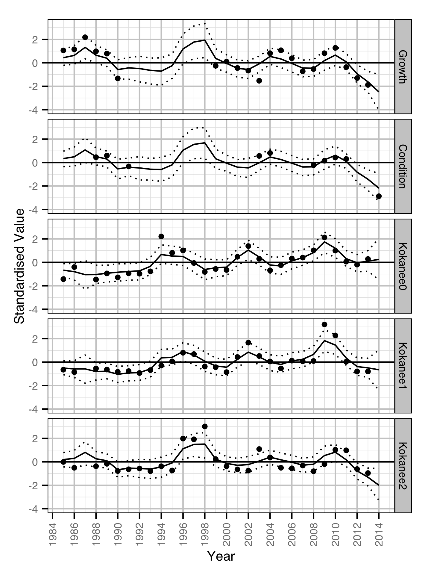
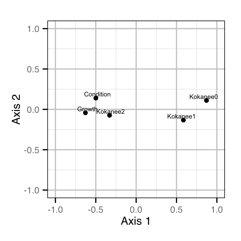
The relative similarities between the yearly condition and growth (scale increment) estimates and the yearly kokanee abundance estimates were estimated using a Dynamic Factor Analysis (Zuur et al. 2003). Due to the rotation problem the underlying trends were indeterminate (Abmann et al. 2014). The growth estimates were lagged by one year.
Key assumptions of the DFA model include:
- The time series are described by two underlying trends.
- The random walk processes in the trends are normally distributed.
- The residual variation in the standardised variables is normally distributed.
Model Code
The JAGS model code, which uses a series of naming conventions, is presented below.
Fecundity
| Variable/Parameter | Description |
|---|---|
bAlpha |
Intercept for log(eFecundity) |
bBeta |
Slope for log(eFecundity[i]) |
Fecundity[i] |
Fecundity of ith fish |
sFecundity |
SD of residual variation in log(Fecundity) |
Fecundity - Model1
model {

  bAlpha ~ dnorm(5, 5^-2)
  bBeta ~ dnorm(1, 5^-2)

  sFecundity ~ dunif(0, 1)
  for(i in 1:length(Fecundity)) {
    log(eFecundity[i]) <- bAlpha + bBeta * Length[i]
    Fecundity[i] ~ dlnorm(log(eFecundity[i]), sFecundity^-2)
  }
}
Condition
| Variable/Parameter | Description |
|---|---|
bAlpha |
Intercept for eAlpha |
bAlphaDayte |
Effect of Dayte on bAlpha |
bAlphaDayte2 |
Quadratic effect of Dayte on bAlpha |
bBeta |
Intercept for eBeta |
Dayte[i] |
Day of the year on which ith fish encountered |
eAlpha |
Predicted intercept for log(eWeight) |
eBeta |
Predicted effect of centred log(Length) on log(eWeight) |
eWeight[i] |
Prediction weight of ith fish |
Length[i] |
Centered log fork length of ith fish |
sAlphaYear |
SD of effect of Year on bAlpha |
sWeight |
SD of residual variation in log(Weight) |
Weight[i] |
Weight of ith fish |
Year[i] |
Year on which ith fish encountered |
Condition - Model1
model {

  bAlpha ~ dnorm(5, 5^-2)
  bBeta ~ dnorm(3, 5^-2)

  bAlphaDayte ~ dnorm(0, 5^-2)
  bAlphaDayte2 ~ dnorm(0, 5^-2)

  sAlphaYear ~ dunif(0, 5)
  for(i in 1:nYear) {
    bAlphaYear[i] ~ dnorm(0, sAlphaYear^-2)
  }

  sWeight ~ dunif(0, 5)
  for(i in 1:length(Weight)) {
    eAlpha[i] <- bAlpha + bAlphaDayte * Dayte[i] + bAlphaDayte2 * Dayte[i]^2 + bAlphaYear[Year[i]]

    eBeta[i] <- bBeta

    log(eWeight[i]) <- eAlpha[i] + eBeta[i] * Length[i]

    Weight[i] ~ dlnorm(log(eWeight[i]), sWeight^-2)
  }
}
Age
| Variable/Parameter | Description |
|---|---|
Age[i] |
Age for ith scale reading |
bK |
Intercept for eK |
bKReader |
Effect of Reader on log(bK) |
bLinf |
Mean maximum length |
bT0Reader |
Effect of Reader on t0 |
eK[i] |
Expected growth coefficient for ith scale reading |
eT0[i] |
Expected length at time zero |
Length[i] |
Fork length at capture for ith scale reading |
Reader[i] |
Reader for ith scale reading |
sKReader |
SD of effect of Fish on bK |
sLength |
SD of residual variation in Length |
t0 |
Intercept for eT0 |
Age - Model1
 model {
  bLInf ~ dunif(700, 1000)
  bK ~ dunif(0, 1)
  t0 ~ dnorm(0, 2^-1)

  bKReader[1] <- 0
  bT0Reader[1] <- 0
  for(i in 2:nReader) {
    bKReader[i] ~ dnorm(0, 1^-2)
    bT0Reader[i] ~ dnorm(0, 5^-2)
  }

  sKFish ~ dunif(0, 1)
  for(i in 1:nFish) {
    bKFish[i] ~ dnorm(0, sKFish^-2)
  }

  sLength ~ dunif(0, 100)
  for (i in 1:length(Length)) {
    eLInf[i] <- bLInf
    log(eK[i]) <- log(bK) + bKReader[Reader[i]] + bKFish[Fish[i]]
    eT0[i] <-  t0 + bT0Reader[Reader[i]]
    eLength[i] <- eLInf[i] * (1 - exp(-eK[i] * (Age[i] - eT0[i])))
    Length[i] ~ dnorm(eLength[i], sLength^-2)
  }
}
Back-Calculated Growth
| Variable/Parameter | Description |
|---|---|
bInc |
Intercept for log(eInc) |
bIncScaleRadius |
Effect of ScaleRadius on bInc |
bIncScaleRadius2 |
Quadratic effect of ScaleRadius on bInc |
bSDInc |
Intercept for log(eSDInc) |
bSDProbability |
Effect of Probability on bSDInc |
eInc[i] |
Expected increment for ith annulus difference |
eSDInc[i] |
Expected SD for for ith annulus difference |
Increment[i] |
Measured annulus difference |
Probability[i] |
Readers minimum confidence in ith annulus difference |
sIncYear |
SD of effect of Year on bInc |
Year[i] |
Inferred year of second annulus for ith annulus difference |
Back-Calculated Growth - Model1
model {

  bInc ~ dnorm(0, 5^-2)
  bIncScaleRadius ~ dnorm(0, 5^-2)
  bIncScaleRadius2 ~ dnorm(0, 5^-2)

  sIncYear ~ dunif(0, 5)
  for (i in 1:nYear) {
    bIncYear[i] ~ dnorm(0, sIncYear^-2)
  }

  bSDInc ~ dnorm(0, 5^-2)
  bSDIncProbability ~ dnorm(0, 5^-2)
  for (i in 1:length(ScaleRadius)) {

    log(eInc[i]) <- bInc + bIncScaleRadius * ScaleRadius[i] + bIncScaleRadius2 * ScaleRadius[i]^2 + bIncYear[Year[i]]

    log(eSDInc[i]) <- bSDInc + bSDIncProbability * Probability[i]

    Increment[i] ~ dlnorm(log(eInc[i]), eSDInc[i]^-2)
  }
}
Dynamic Factor Analysis
| Variable/Parameter | Description |
|---|---|
bDistance[i,j] |
Euclidean distance between ith and jth Variable |
bTrendYear[t,y] |
Expected value for tth trend in yth Year |
eValue[v,y,t] |
Expected standardised value for vth Variable in yth Year considering tth trends |
sTrend |
SD in trend random walks |
sValue |
SD for residual variation in Value |
Value[i] |
Standardised value for ith data point |
Variable[i] |
Variable for ith data point |
Year[i] |
Year of ith data point |
Z[v,y] |
Expected weighting for vth Variable in yth Year |
Dynamic Factor Analysis - Model1
model{

  sTrend ~ dunif(0, 1)
  for (t in 1:nTrend) {
    bTrendYear[t,1] ~ dunif(-1,1)
    for(y in 2:nYear){
      bTrendYear[t,y] ~ dnorm(bTrendYear[t,y-1], sTrend^-2)
    }
  }

  for(v in 1:nVariable){
    for(t in 1:nTrend) {
      Z[v,t] ~ dunif(-1,1)
    }
    for(y in 1:nYear){
      eValue[v,y,1] <- Z[v,1] * bTrendYear[1,y]
      for(t in 2:nTrend) {
        eValue[v,y,t] <- eValue[v,y,t-1] + Z[v,t] * bTrendYear[t,y]
      }
    }
  }

  sValue ~ dunif(0, 1)
  for(i in 1:length(Value)) {
    Value[i] ~ dnorm(eValue[Variable[i], Year[i], nTrend], sValue^-2)
  }

  for(i in 1:nVariable) {
    for(j in 1:nVariable) {
      bDistance[i,j] <- sqrt(sum((Z[i,]-Z[j,])^2))
    }
  }
}
Results
Model Parameters
The posterior distributions for the fixed (Kery and Schaub 2011 p. 75) parameters in each model are summarised below.
Fecundity
| Parameter | Estimate | Lower | Upper | SD | Error | Significance |
|---|---|---|---|---|---|---|
| bAlpha | 8.97374 | 8.93630 | 9.01392 | 0.01892 | 0 | 7e-04 |
| bBeta | 1.74870 | 1.40080 | 2.10560 | 0.17440 | 20 | 7e-04 |
| sFecundity | 0.07758 | 0.05576 | 0.11355 | 0.01439 | 37 | 7e-04 |
| Convergence | Iterations |
|---|---|
| 1.01 | 1000 |
Condition
| Parameter | Estimate | Lower | Upper | SD | Error | Significance |
|---|---|---|---|---|---|---|
| bAlpha | 1.32120 | 1.25860 | 1.39270 | 0.03270 | 5 | 0.0010 |
| bAlphaDayte | -0.01217 | -0.02538 | 0.00124 | 0.00677 | 110 | 0.0739 |
| bAlphaDayte2 | 0.02240 | 0.01008 | 0.03431 | 0.00610 | 54 | 0.0010 |
| bBeta | 3.26010 | 3.18960 | 3.32970 | 0.03690 | 2 | 0.0010 |
| sAlphaYear | 0.10060 | 0.06010 | 0.16500 | 0.02690 | 52 | 0.0010 |
| sWeight | 0.15795 | 0.15059 | 0.16647 | 0.00400 | 5 | 0.0010 |
| Convergence | Iterations |
|---|---|
| 1.01 | 1e+05 |
Age
| Parameter | Estimate | Lower | Upper | SD | Error | Significance |
|---|---|---|---|---|---|---|
| bK | 0.17204 | 0.15224 | 0.19128 | 0.01034 | 11 | 0.0010 |
| bKReader[2] | -0.03520 | -0.08910 | 0.02140 | 0.02790 | 160 | 0.1827 |
| bKReader[3] | 0.61110 | 0.49270 | 0.72450 | 0.06070 | 19 | 0.0010 |
| bLInf | 924.18000 | 904.69000 | 951.64000 | 11.83000 | 3 | 0.0010 |
| bT0Reader[2] | -0.19280 | -0.50200 | 0.09670 | 0.15340 | 160 | 0.2129 |
| bT0Reader[3] | 2.10600 | 1.52600 | 2.81600 | 0.32800 | 31 | 0.0010 |
| sKFish | 0.32669 | 0.29840 | 0.35558 | 0.01470 | 9 | 0.0010 |
| sLength | 20.59600 | 17.63400 | 23.95700 | 1.54000 | 15 | 0.0010 |
| t0 | -0.85200 | -1.64400 | -0.28300 | 0.34900 | 80 | 0.0010 |
| Convergence | Iterations |
|---|---|
| 1.04 | 80000 |
Back-Calculated Growth
| Parameter | Estimate | Lower | Upper | SD | Error | Significance |
|---|---|---|---|---|---|---|
| bInc | 1.59690 | 1.52200 | 1.66850 | 0.03780 | 5 | 0.0010 |
| bIncScaleRadius | 0.16324 | 0.13690 | 0.19196 | 0.01453 | 17 | 0.0010 |
| bIncScaleRadius2 | -0.09418 | -0.11742 | -0.07253 | 0.01144 | 24 | 0.0010 |
| bSDInc | -0.96289 | -1.00488 | -0.91875 | 0.02153 | 4 | 0.0010 |
| bSDIncProbability | 0.02469 | -0.01958 | 0.06840 | 0.02263 | 180 | 0.2595 |
| sIncYear | 0.14790 | 0.09810 | 0.22190 | 0.03150 | 42 | 0.0010 |
| Convergence | Iterations |
|---|---|
| 1.01 | 1e+05 |
Dynamic Factor Analysis
| Parameter | Estimate | Lower | Upper | SD | Error | Significance |
|---|---|---|---|---|---|---|
| sTrend | 0.7754 | 0.4984 | 0.9807 | 0.1311 | 31 | 0.001 |
| sValue | 0.6182 | 0.5053 | 0.7812 | 0.0694 | 22 | 0.001 |
| Convergence | Iterations |
|---|---|
| 1.02 | 1e+05 |
Figures
Condition
Age
Back-Calculated Growth
Dynamic Factor Analysis
Acknowledgements
The organisations and individuals whose contributions have made this analysis report possible include:
- Birkenhead Scale Analyses
- Carol Lidstone
- Reel Adventures
- Kerry Reed
- Les Fleck