Kettle and Granby Rivers Adult Rainbow Trout Density Analysis 2017
The suggested citation for this analytic report is:
Thorley, J.L. and Dalgarno S. (2018) Kettle and Granby Rivers Adult Rainbow Trout Density Analysis 2017. A Poisson Consulting Analysis Report. URL: https://www.poissonconsulting.ca/f/6124688.
Background
The Kettle drainage consists of the West Kettle River, the Kettle River and the Granby River sub-basins.
The primary goal of the current analysis report is to answer the following question:
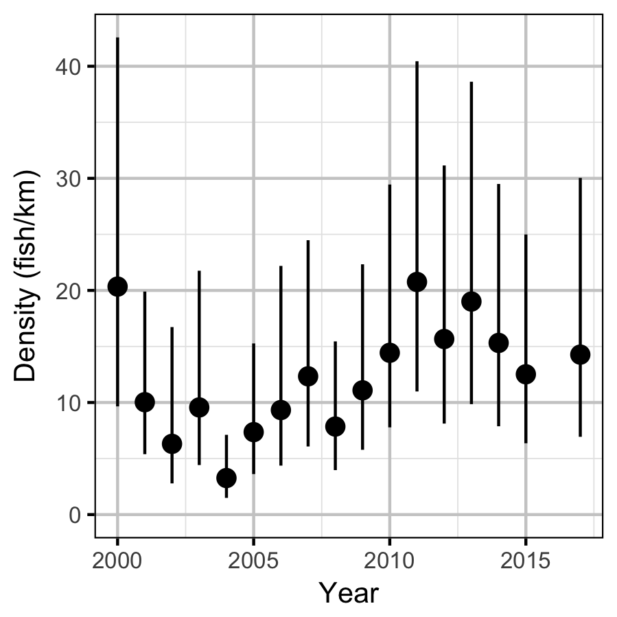
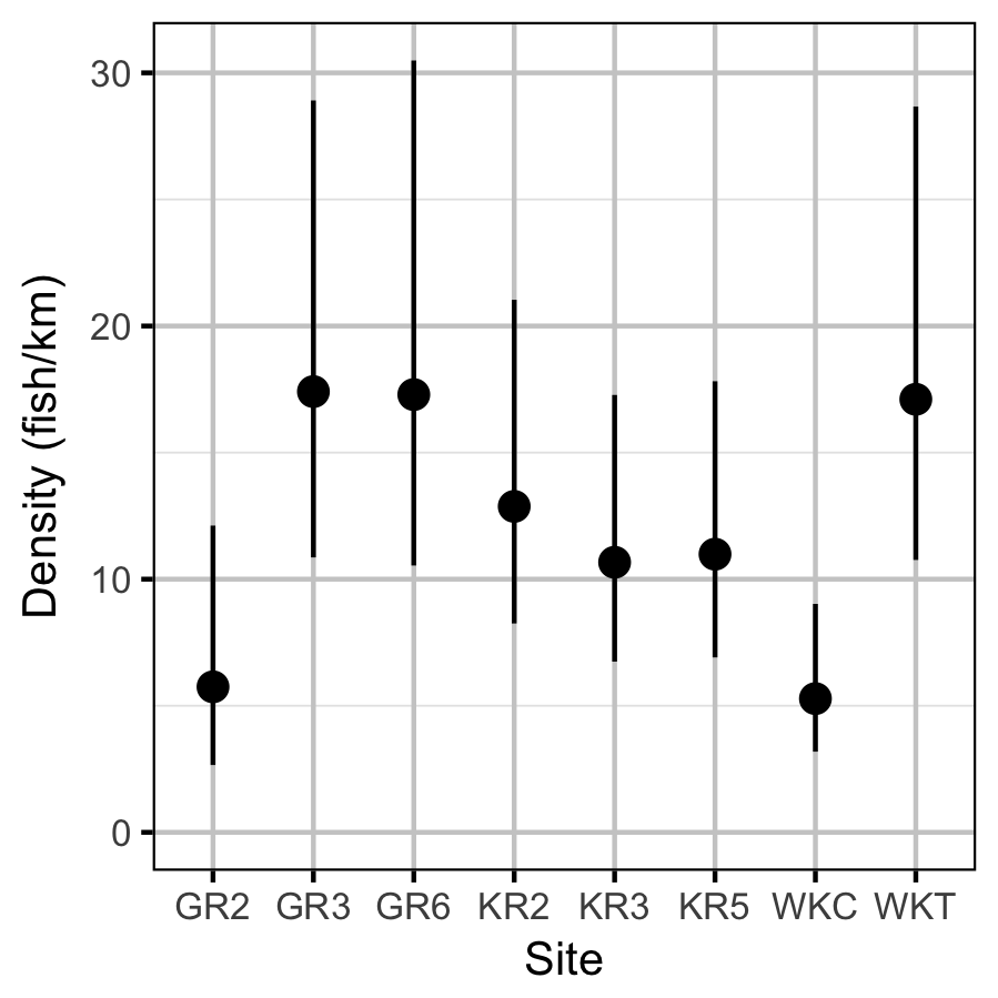
What are the annual densities of Rainbow Trout at each of the index sites and how have they changed through time?
Data Preparation
The data were provided in the form of an Access database. The data were rearchived in an SQLite database and prepared for analysis using R version 3.5.0 (R Core Team 2018).
Statistical Analysis
Model parameters were estimated using Bayesian methods. The Bayesian estimates were produced using JAGS (Plummer 2015). For additional information on Bayesian estimation the reader is referred to McElreath (2016).
Unless indicated otherwise, the Bayesian analyses used normal and uniform prior distributions that did not constrain the posteriors (Kery and Schaub 2011, 36). The posterior distributions were estimated from 1500 Markov Chain Monte Carlo (MCMC) samples thinned from the second halves of 3 chains (Kery and Schaub 2011, 38–40). Model convergence was confirmed by ensuring that \(\hat{R} \leq 1.05\) (Kery and Schaub 2011, 40) and \(\textrm{ESS} \geq 150\) for each of the monitored parameters (Kery and Schaub 2011, 61). Where \(\hat{R}\) is the potential scale reduction factor and \(\textrm{ESS}\) is the effective sample size (Brooks et al. 2011).
The parameters are summarised in terms of the point estimate, standard deviation (sd), the z-score, lower and upper 95% confidence/credible limits (CLs) and the p-value (Kery and Schaub 2011, 37, 42). The estimate is the median (50th percentile) of the MCMC samples, the z-score is \(\mathrm{mean}/\mathrm{sd}\) and the 95% CLs are the 2.5th and 97.5th percentiles. A p-value of 0.05 indicates that the lower or upper 95% CL is 0.
Where relevant, model adequacy was confirmed by examination of residual plots for the full model(s).
The results are displayed graphically by plotting the modeled relationships between particular variables and the response(s) with the remaining variables held constant. In general, continuous and discrete fixed variables are held constant at their mean and first level values, respectively, while random variables are held constant at their typical values (expected values of the underlying hyperdistributions) (Kery and Schaub 2011, 77–82). When informative the influence of particular variables is expressed in terms of the effect size (i.e., percent change in the response variable) with 95% confidence/credible intervals (CIs, Bradford, Korman, and Higgins 2005).
The analyses were implemented using R version 3.5.0
(R Core Team 2018) and the
mbr family of packages.
Model Descriptions
Density
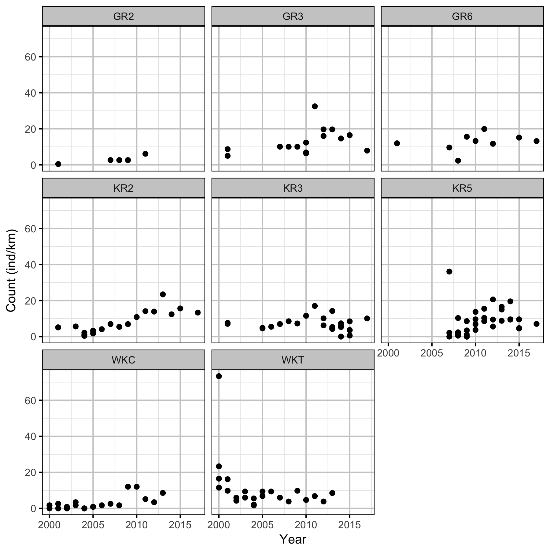
The lineal density and observer efficiency for Rainbow \(\geq\) 30 cm in length were estimated from the snorkel count and mark-resighting data for the Kettle River using an overdispersed Poisson mark-recapture model.
Key assumptions of the density model include:
- Density varies randomly by year and site.
- The number of resighted individuals is described by a binomial distribution where the probability of resighting is the observer efficiency.
- The expected number of observed individuals is the product of the density, site length, proportion of the site surveyed and the observer efficiency.
- The number of observed individuals is described by a gamma-Poisson distribution.
Model Templates
Density
model {
  bEfficiency ~ dunif(0, 1)

  bDensity ~ dnorm(5, 2^-2)

  sDensityAnnual ~ dunif(0, 1)
  for (yr in 1:nAnnual) {
    bDensityAnnual[yr] ~ dnorm(0, sDensityAnnual^-2)
  }

  sDensitySite ~ dunif(0, 2)
  for (i in 1:nSite) {
    bDensitySite[i] ~ dnorm(0, sDensitySite^-2)
  }

  sDispersion ~ dunif(0, 1)
  for (i in 1:length(Count)) {

    eEfficiency[i] <- bEfficiency
    eResightingEfficiency[i] <- min(eEfficiency[i], Marked[i])

    eAdjustedMarked[i] <- max(Marked[i], 1)
    Resighted[i] ~ dbin(eResightingEfficiency[i] * ProportionSurveyed[i], eAdjustedMarked[i])

    log(eDensity[i]) <- bDensity + bDensityAnnual[Annual[i]] + bDensitySite[Site[i]]
    eAbundance[i] <- eDensity[i] * SiteLength[i]
    eDispersion[i] ~ dgamma(1 / sDispersion^2, 1 / sDispersion^2)
    Count[i] ~ dpois(eAbundance[i] * eEfficiency[i] * ProportionSurveyed[i] * eDispersion[i])
  }
..
Template 1. The model description.
Results
Tables
Density
Table 1. Parameter descriptions.
| Parameter | Description |
|---|---|
Annual[i] |
Year of ith site visit as a factor |
bDensity |
Intercept of log(eDensity) |
bDensityAnnual[i] |
Effect of ith year on bDensity |
bDensitySite[i] |
Effect of ith site on bDensity |
bEfficiency |
Intercept for logit(eEfficiency) |
Count[i] |
Number of fish observed during the ith site
visit |
eAbundance[i] |
Expected abundance during ith site visit |
eDensity[i] |
Expected fish density during the ith site
visit |
eEfficiency[i] |
Expected observer efficiency during the ith
site visit |
Marked[i] |
Number of fish marked prior to the ith site
visit |
ProportionSurveyed[i] |
Proportion of site surveyed during the ith
site visit |
Resighted[i] |
Number of marked fish observed during the ith
site visit |
sDensityAnnual |
SD of bDensityAnnual |
sDensitySite |
SD of bDensitySite |
SiteLength[i] |
Length of the site visited for the ith site
visit |
Table 2. Model coefficients.
| term | estimate | sd | zscore | lower | upper | pvalue |
|---|---|---|---|---|---|---|
| bDensity | 2.4428815 | 0.3129692 | 7.806787 | 1.8145873 | 3.0677045 | 7e-04 |
| bEfficiency | 0.6004595 | 0.0769296 | 7.748800 | 0.4378218 | 0.7334505 | 7e-04 |
| sDensityAnnual | 0.5489974 | 0.1283577 | 4.372507 | 0.3497721 | 0.8490307 | 7e-04 |
| sDensitySite | 0.5790858 | 0.2368565 | 2.636561 | 0.3059285 | 1.2032050 | 7e-04 |
| sDispersion | 0.5771703 | 0.0515824 | 11.258111 | 0.4883693 | 0.6891421 | 7e-04 |
Table 3. Model summary.
| n | K | nchains | niters | nthin | ess | rhat | converged |
|---|---|---|---|---|---|---|---|
| 149 | 5 | 3 | 500 | 100 | 300 | 1.009 | TRUE |
Figures
Density


Acknowledgements
The organisations and individuals whose contributions have made this analysis report possible include:
- Habitat Conservation Trust Foundation and the anglers, hunters, trappers and guides who contribute to the Trust
- Ministry of Forests, Lands and Natural Resource
Operations
- Tara White
- Greg Andrusak
- Greg Wilson
- Hilary Ward
- Rob Bison
- Gerry Oliver
- Terry Anderson
- Herb Tepper
- Gary Pavan
- Vicky Lipinski
- Ken Ashley
- Pat Slaney
- Paul Askey
- Stefan Himmer
- Robyn Irvine
- Jimmy Robbins
- Alan Caverley
- Brian Janz
- Christian St.Pierre
- Dean Watts
- Heather Deal
- Jerry Mitchell
- Steve Matthews
- Wendell Koning
- Phil Epp
- Aaron Reid
- Erin Reid
- Andrew Wilson
- Sherri McPhersen
- Andrew Walker
- Eric Hegerat
- Chris White
- Ryan Whitehouse
References
Bradford, Michael J, Josh Korman, and Paul S Higgins. 2005. “Using Confidence Intervals to Estimate the Response of Salmon Populations (Oncorhynchus Spp.) to Experimental Habitat Alterations.” Canadian Journal of Fisheries and Aquatic Sciences 62 (12): 2716–26. https://doi.org/10.1139/f05-179.
Brooks, Steve, Andrew Gelman, Galin L. Jones, and Xiao-Li Meng, eds. 2011. Handbook for Markov Chain Monte Carlo. Boca Raton: Taylor & Francis.
Kery, Marc, and Michael Schaub. 2011. Bayesian Population Analysis Using WinBUGS : A Hierarchical Perspective. Boston: Academic Press. http://www.vogelwarte.ch/bpa.html.
McElreath, Richard. 2016. Statistical Rethinking: A Bayesian Course with Examples in R and Stan. Chapman & Hall/CRC Texts in Statistical Science Series 122. Boca Raton: CRC Press/Taylor & Francis Group.
Plummer, Martyn. 2015. “JAGS Version 4.0.1 User Manual.” http://sourceforge.net/projects/mcmc-jags/files/Manuals/4.x/.
R Core Team. 2018. R: A Language and Environment for Statistical Computing. Vienna, Austria: R Foundation for Statistical Computing. https://www.R-project.org/.