Kaslo Bull Trout Productivity 2021
The suggested citation for this analytic appendix is:
Thorley, J.L., Andrusak, G.F. and Amies-Galonski, E. (2022) Kaslo Bull Trout Productivity 2021. A Poisson Consulting Analytic Appendix. URL: https://www.poissonconsulting.ca/f/433821282.
Background
The Kaslo River and Keen Creek, which is a tributary of the Kaslo River, are important Bull Trout spawning and rearing tributaries on Kootenay Lake. From 2012 to 2021, field crews have night-snorkeled these systems in the fall and recorded all Bull Trout less than 350 mm in length. Keen Creek was not snorkelled in 2020 or 2021 due to visibility issues. Snorkel and electrofishing marking crews have also captured and tagged juvenile Bull Trout for the snorkel crews to resight. Redd counts have been conducted in both systems since 2006, with the exception of 2020 and 2021, when Keen Creek was not surveyed. The primary goal of the current analyses is to answer the following questions:
What is the observer efficiency when night-snorkeling for juvenile Bull Trout in the Kaslo River and Keen Creek?
What are the numbers of age-1 Bull Trout in the Kaslo River and Keen Creek?
What is the relationship between the stock (number of redds and eggs) and the resultant numbers of age-1 Bull Trout two years later?
Data Preparation
The data were cleaned, tidied and databased using R version 4.2.1 (R Core Team 2015).
Statistical Analysis
Model parameters were estimated using Bayesian methods. The Bayesian estimates were produced using JAGS (Plummer 2015). For additional information on Bayesian estimation the reader is referred to McElreath (2016).
Unless indicated otherwise, the Bayesian analyses used weakly informative normal or truncated half normal prior distributions (Kery and Schaub 2011, 36). The posterior distributions were estimated from 1500 Markov Chain Monte Carlo (MCMC) samples thinned from the second halves of 3 chains (Kery and Schaub 2011, 38–40). Model convergence was confirmed by ensuring that \(\hat{R} \leq\) 1.05 (Kery and Schaub 2011, 40) and \(\textrm{ESS} \geq 150\) for each of the monitored parameters (Kery and Schaub 2011, 61). Where \(\hat{R}\) is the potential scale reduction factor and \(\textrm{ESS}\) is the effective sample size.
The parameters are summarised in terms of the point estimate, lower and upper 95% credible limits (CLs) and the surprisal s-value (Greenland 2019). The estimate is the median (50th percentile) of the MCMC samples while the 95% CLs are the 2.5th and 97.5th percentiles. The s-value can be considered a test of directionality. More specifically it indicates how surprising (in bits) it would be to discover that the true value of the parameter is in the opposite direction to the estimate. An s-value of 4.3 bits, which is equivalent to a p-value (Kery and Schaub 2011; Greenland and Poole 2013) of 0.05, indicates that the surprise would be equivalent to throwing 4.3 heads in a row.
Where relevant, model adequacy was confirmed by examination of residual plots for the full model(s).
The results are displayed graphically by plotting the modeled relationships between particular variables and the response(s) with the remaining variables held constant. In general, continuous and discrete fixed variables are held constant at their mean and first level values, respectively, while random variables are held constant at their typical values (expected values of the underlying hyperdistributions) (Kery and Schaub 2011, 77–82). When informative the influence of particular variables is expressed in terms of the effect size (i.e., percent change in the response variable) with 95% confidence/credible intervals (CIs, Bradford et al. 2005).
The analyses were implemented using R version 4.2.1
(R Core Team 2015) and the
mbr family of packages.
Model Descriptions
Length Correction
The annual bias (inaccuracy) and error (imprecision) in observer’s fish length estimates when spotlighting (standing) and snorkeling were quantified from the divergence of their length distribution from the length distribution for JLT and SH (the two most experience snorkelers) in that year. More specifically, the length correction that minimised the Jensen-Shannon divergence (Lin 1991) provided a measure of the inaccuracy while the minimum divergence (the Jensen-Shannon divergence was calculated with log to base 2 which means it lies between 0 and 1) provided a measure of the imprecision.
Observer Efficiency
All resighted fish with a tag were allocated to the closest unallocated marked fish (with the same colour tag) by fork length and distance. The marked fish were analysed using a Bayesian logistic regression model. The key assumption of the logistic regression model is that:
- The observer efficiency varies by the fork length.
The preliminary analysis for observer efficiency indicated that system, observer, gradient, sinuosity, and river kilometre were not informative predictors.
Lineal Density
Both systems were broken into 100 m sites by bank. The lineal density at each site was estimated using an over-dispersed Poisson Generalized Linear Mixed Model.
Key assumptions of the Bayesian GLMM include:
- The lineal density varies between systems and years.
- The lineal density varies randomly by site.
- The observer efficiency for each system is as estimated by the observer efficiency model.
The preliminary analysis for density indicated that site sinuosity, gradient, and river kilometre were not informative predictors.
Redds Stock-Recruitment
The stock-recruitment relationship was estimated using a Bayesian Beverton-Holt stock-recruitment curve. Key assumptions of the final BH SR model include:
- The strength of density-dependence varies between systems.
- The residual variation is log normally distributed.
The \(E_{K/2}\) Limit Reference Point (Mace 1994) (\(E_{0.5 R_{max}}\)) was calculated, corresponding to the stock (number of redds per kilometer) that produce 50% of the maximum recruitment (\(K\)).
Condition
The condition of adults was estimated using an allometric weight-length relationship. Key assumptions of the condition model include:
- Condition varies randomly by year.
- The residual variation in weight is log normally distributed.
Fecundity
Female spawner fecundity was estimated using an allometric egg-weight relationship. The key assumption of the fecundity model is that:
- The residual variation in fecundity is log normally distributed.
Spawner Length
The average length of spawners in each system and year was estimated using a linear regression. Key assumptions of the spawner length model include:
- Length varies randomly with system, year, and system within year.
- The residual variation is normally distributed.
Egg Deposition
The total egg deposition in each year was estimated by
- Converting the average spawner length to the average weight using the condition relationship for a typical year.
- Adjusting the average weight by the annual condition effect (interpolating where unavailable)
- Converting the average weight to the average fecundity using the fecundity relationship
- Multiplying the average fecundity by the number of females (assuming 1 female per redd)
Eggs Stock-Recruitment
The stock-recruitment relationship between the total number eggs and the abundance of age-1 individuals was estimated using a Bayesian Beverton-Holt stock-recruitment curve. Key assumptions of the final BH SR model include:
- The prior uncertainty in the egg to age-1 survival is described by a Beta distribution with an alpha of 4 and beta of 49 which has a mean of 0.075 and a standard deviation of 0.036. This is based off the assumption that a recruit has a ~50% chance of surviving through each summer or winter and must pass through two winters and two summers to survive to age-1.
- The carrying capacity varies between systems.
- The residual variation in the recruits is log normally distributed.
The \(E_{K/2}\) Limit Reference Point (Mace 1994) (\(E_{0.5 R_{max}}\)) was calculated, corresponding to the stock (number of eggs per 100 meters) that produce 50% of the maximum recruitment (\(K\)).
Model Templates
Observer Efficiency
model{
  bIntercept ~ dnorm(0, 2^-2)
  bLength ~ dnorm(0, 2^-2)

  for(i in 1:length(Observed)){
    logit(eObserved[i]) <-  bIntercept + bLength * Length[i]
    Observed[i] ~ dbern(eObserved[i])
  }
Block 1. Final model.
Lineal Density
model{
  bEfficiency ~ dnorm(Efficiency[1], EfficiencySD[1]^-2) T(0, 1)

  b0 ~ dnorm(0, 5^-2)
  bRkm ~ dnorm(0, 2^-2)
  bSystem[1] <- 0
  for(i in 2:nSystem) {
    bSystem[i] ~ dnorm(0, 2^2)
  }

  sSystemYear ~ dnorm(0, 2^-2) T(0,)
  for(i in 1:nSystem) {
    for(j in 1:nYear) {
      bSystemYear[i,j] ~ dnorm(0, sSystemYear^-2)
    }
  }

  sSite ~ dnorm(0, 2^-2) T(0,)
  for(i in 1:nSite) {
    bSite[i] ~ dnorm(0, sSite^-2)
  }

  sDispersion ~ dnorm(0, 2^-2) T(0,)
  for(i in 1:length(Count)) {
    log(eDensity[i]) <- b0 + bSystem[System[i]] + bRkm * Rkm[i] + bSite[Site[i]] + bSystemYear[System[i],Year[i]]
    eDispersion[i] ~ dgamma(sDispersion^-2, sDispersion^-2)
    Count[i] ~ dpois(eDensity[i] * Length[i] * Coverage[i] * bEfficiency * eDispersion[i])
  }
Block 2. The final model.
Redds Stock-Recruiment
model {
  log_bAlpha ~ dnorm(5, 5^-2)
  log(bAlpha) <- log_bAlpha

  for(i in 1:nSystem) {
    log_bBeta[i] ~ dnorm(0, 5^-2)
    log(bBeta[i]) <- log_bBeta[i]
  }

  log_sRecruits ~ dnorm(0, 5^-2)
  log(sRecruits) <- log_sRecruits

  for(i in 1:length(Recruits)){
    eRecruits[i] <- bAlpha * Stock[i] / (1 + bBeta[System[i]] * Stock[i])
    Recruits[i] ~ dlnorm(log(eRecruits[i]), sRecruits^-2)
  }
  bCarryingCapacity <- bAlpha / bBeta
Block 3. Final model.
Condition
model{
  b0 ~ dnorm(6, 2^-2)
  bLength ~ dnorm(3, 1^-2)
  sWeight ~ dnorm(0, 1^-2) T(0,)
  sYear ~ dnorm(0, 1^-2) T(0,)

  for (i in 1:nYear) {
    bYear[i] ~ dnorm(0, sYear^-2)
  }

  for (i in 1:nObs) {
    log(eWeight[i]) <- b0 + (log(Length[i]) - log(500)) * bLength + bYear[Year[i]]
    Weight[i] ~ dlnorm(log(eWeight[i]), sWeight^-2)
  }
Block 4. Model description.
Fecundity
model{
  b0 ~ dnorm(0, 2^-2)
  bWeight ~ dnorm(1, 2^-2)
  sFecundity ~ dnorm(0, 2^-2) T(0,)

  for (i in 1:nObs) {
    log(eFecundity[i]) <- b0 + (log(Weight[i]) - log(2300)) * bWeight
    Fecundity[i] ~ dlnorm(log(eFecundity[i]), sFecundity^-2)
  }
Block 5. Model description.
Spawner Length
model{
  bLength ~ dnorm(650, 100^-2)
  sLength ~ dnorm(0, 100^-2) T(0,)
  sYear ~ dnorm(0, 100^-2) T(0,)
  sSystem ~ dnorm(0, 100^-2) T(0,)
  sYearSystem ~ dnorm(0, 100^-2) T(0,)
  bSex ~ dbeta(1, 1)
  bFemale ~ dnorm(0, 100^-2)
  bBias ~ dnorm(0, 100^-2)

  for (i in 1:nYear) {
    bYear[i] ~ dnorm(0, sYear^-2)
  }

  for (i in 1:nSystem) {
    bSystem[i] ~ dnorm(0, sSystem^-2)
  }

  for (i in 1:nYear) {
    for (j in 1:nSystem) {
        bYearSystem[i, j] ~ dnorm(0, sYearSystem^-2)
    }
  }

  bCatchType[1] <- 0
  for(i in 2:nCatchType) {
    bCatchType[i] ~ dnorm(0, 100^-2)
  }

  for (i in 1:nObs) {
    Female[i] ~ dbern(bSex)
    eLength[i] <- bLength + bSystem[System[i]] + bFemale * Female[i] + bCatchType[CatchType[i]] + bYear[Year[i]] + bYearSystem[Year[i], System[i]] + bBias * Bias[i]
    Length[i] ~ dnorm(eLength[i], sLength^-2)
  }
Block 6. Model description.
Eggs Stock-Recruiment
model {
  bAlpha ~ dbeta(4, 49)

  bK ~ dnorm(3, 1^-2)
  bKPopulation ~ dnorm(0, 1^-2)
  sRecruits ~ dexp(1)

  for(i in 1:nObs){
    log(eK[i]) <- bK + (Kaslo[i] * bKPopulation - (1-Kaslo[i]) * bKPopulation)
    eBeta[i] <-  bAlpha/eK[i]
    eRecruits[i] <- bAlpha * Stock[i] / (1 + eBeta[i] * Stock[i])
    Recruits[i] ~ dlnorm(log(eRecruits[i]), sRecruits^-2)
  }
Block 7. Final model.
Results
Tables
Coverage
Table 1. Total length of river bank counted (including replicates) by system and year.
| System | Year | Length (km) |
|---|---|---|
| Kaslo River | 2012 | 10.57 [km] |
| Kaslo River | 2013 | 13.43 [km] |
| Kaslo River | 2014 | 11.45 [km] |
| Kaslo River | 2015 | 7.32 [km] |
| Kaslo River | 2016 | 11.59 [km] |
| Kaslo River | 2017 | 9.79 [km] |
| Kaslo River | 2018 | 8.44 [km] |
| Kaslo River | 2019 | 7.19 [km] |
| Kaslo River | 2020 | 10.42 [km] |
| Kaslo River | 2021 | 11.08 [km] |
| Keen Creek | 2012 | 1.44 [km] |
| Keen Creek | 2013 | 0.95 [km] |
| Keen Creek | 2014 | 0.67 [km] |
| Keen Creek | 2015 | 0.72 [km] |
| Keen Creek | 2016 | 0.85 [km] |
| Keen Creek | 2017 | 1.68 [km] |
| Keen Creek | 2018 | 3.37 [km] |
| Keen Creek | 2019 | 1.48 [km] |
Observer Efficiency
Table 2. Parameter descriptions.
| Parameter | Description |
|---|---|
bIntercept |
The intercept for logit(eObserved) |
bLength |
The effect of Length on bIntercept |
bLength2 |
The effect of Length on the effect of Length on
bIntercept |
eObserved |
The expected probability of observing an individual |
Length |
The standardized fork length |
Observed |
The number of individuals observed (0 or 1) |
Tagged |
The number of tagged individuals (1) |
Table 3. Final parameter estimates.
| term | estimate | lower | upper | svalue |
|---|---|---|---|---|
| bIntercept | -1.4487570 | -1.8123174 | -1.126471 | 10.55171 |
| bLength | 0.6744263 | 0.3223635 | 1.047922 | 10.55171 |
Table 4. Observer Efficiency estimates for a 123 mm Bull Trout.
| System | Efficiency | EfficiencyLower | EfficiencyUpper | EfficiencySD |
|---|---|---|---|---|
| Kaslo River | 0.1517101 | 0.1021055 | 0.2103352 | 0.0276096 |
Table 5. Final model summary.
| n | K | nchains | niters | nthin | ess | rhat | converged |
|---|---|---|---|---|---|---|---|
| 220 | 2 | 3 | 500 | 1 | 656 | 1 | TRUE |
Lineal Density
Table 6. Parameter descriptions.
| Parameter | Description |
|---|---|
bDispersion |
The random effect of overdispersion |
bSite |
The random effect of Site on bSystemYear |
bSystemYear |
The effect of System and Year on log(eDensity) |
Count |
Number of fish counted |
Coverage |
Proportion of site surveyed |
Dispersion |
Factor for random effect of overdispersion |
eCount |
The expected Count |
eDensity |
The expected lineal density |
Efficiency |
The observer efficiency from the observer efficiency model |
Length |
Length of site (m) |
log_sDispersion |
log(sDispersion) |
log_sSite |
log(sSite) |
sDispersion |
The SD of bDispersion |
Site |
The site |
sSite |
The SD of bSite |
System |
The system |
Year |
The year |
Table 7. Parameter estimates.
| term | estimate | lower | upper | svalue |
|---|---|---|---|---|
| b0 | -2.5782529 | -3.0153014 | -2.0765395 | 10.55171 |
| bEfficiency | 0.1501718 | 0.0964656 | 0.2044709 | 10.55171 |
| bRkm | 0.4303969 | 0.3320728 | 0.5315148 | 10.55171 |
| bSystem[1] | 0.0000000 | 0.0000000 | 0.0000000 | 0.00000 |
| bSystem[2] | 0.9893620 | 0.4743176 | 1.4096555 | 10.55171 |
| sSystemYear | 0.3905191 | 0.2415141 | 0.6489998 | 10.55171 |
Table 8. Model summary.
| n | K | nchains | niters | nthin | ess | rhat | converged |
|---|---|---|---|---|---|---|---|
| 1221 | 5 | 3 | 500 | 50 | 302 | 1.006 | TRUE |
Redds Stock-Recruiment
Table 9. Parameter descriptions.
| Parameter | Description |
|---|---|
Recruits |
Age-1 Bull Trout density |
Stock |
Bull Trout redd density |
bBeta |
Density-dependence |
eRecruits |
Expected density of Recruits |
bAlpha |
Recruits per stock per kilometer at low stock density |
sRecruits |
SD of residual variation in Recruits |
Table 10. Final parameter estimates.
| term | estimate | lower | upper | svalue |
|---|---|---|---|---|
| bAlpha | 198.2745112 | 64.2477732 | 25986.3439344 | 10.5517083 |
| bBeta[1] | 1.1486360 | 0.2806631 | 162.3587450 | 10.5517083 |
| bBeta[2] | 0.6243653 | 0.1160571 | 95.7042676 | 10.5517083 |
| bCarryingCapacity[1] | 176.3135299 | 136.6966818 | 242.0315986 | 10.5517083 |
| bCarryingCapacity[2] | 318.7745433 | 227.8991514 | 553.8778991 | 10.5517083 |
| log_bAlpha | 5.2896523 | 4.1627380 | 10.1638304 | 10.5517083 |
| log_bBeta[1] | 0.1385749 | -1.2706013 | 5.0890772 | 0.1583178 |
| log_bBeta[2] | -0.4710197 | -2.1537069 | 4.5604112 | 0.5531178 |
| log_sRecruits | -1.1799035 | -1.5082235 | -0.7629883 | 10.5517083 |
| sRecruits | 0.3073084 | 0.2213028 | 0.4662715 | 10.5517083 |
Table 11. Final model summary.
| n | K | nchains | niters | nthin | ess | rhat | converged |
|---|---|---|---|---|---|---|---|
| 18 | 10 | 3 | 500 | 100 | 174 | 1.029 | TRUE |
Table 12. Ek/2 Limit Reference Point estimates.
| System | estimate | lower | upper | svalue |
|---|---|---|---|---|
| Kaslo River | 0.8705982 | 0.0061682 | 3.562998 | 10.55171 |
| Keen Creek | 1.6016265 | 0.0104667 | 8.617035 | 10.55171 |
Condition
Table 13. Parameter descriptions.
| Parameter | Description |
|---|---|
b0 |
Intercept for eLength |
bLength |
The effect of Length on eWeight |
bYear[i] |
The effect of year on eWeight |
eWeight[i] |
Expected value of Weight[i] |
Length[i] |
The ith Length value |
sWeight |
SD of residual variation in Weight |
sYear |
SD of Year |
Weight[i] |
The ith Weight value |
Year[i] |
The ith Year value |
Table 14. Model coefficients.
| term | estimate | lower | upper | svalue |
|---|---|---|---|---|
| b0 | 7.0915667 | 6.9948741 | 7.1891419 | 10.55171 |
| bLength | 2.9162213 | 2.8563706 | 2.9762244 | 10.55171 |
| sWeight | 0.1287059 | 0.1224407 | 0.1352182 | 10.55171 |
| sYear | 0.1067360 | 0.0622920 | 0.2333023 | 10.55171 |
Table 15. Model convergence.
| n | K | nchains | niters | nthin | ess | rhat | converged |
|---|---|---|---|---|---|---|---|
| 795 | 4 | 3 | 500 | 50 | 180 | 1.021 | TRUE |
Table 16. Model posterior predictive checks.
| moment | observed | median | lower | upper | svalue |
|---|---|---|---|---|---|
| zeros | NA | NA | NA | NA | NA |
| mean | -0.0007750 | 0.0006637 | -0.0694989 | 0.0687595 | 0.0468893 |
| variance | 0.9884704 | 0.9971119 | 0.9001576 | 1.1057903 | 0.2018742 |
| skewness | -0.4451947 | 0.0024868 | -0.1747122 | 0.1788297 | 10.5517083 |
| kurtosis | 1.7347196 | -0.0124641 | -0.3155986 | 0.3739763 | 10.5517083 |
Table 17. Model sensitivity.
| n | K | nchains | niters | rhat_1 | rhat_2 | rhat_all | converged |
|---|---|---|---|---|---|---|---|
| 795 | 4 | 3 | 500 | 1.021 | 1.005 | 1.014 | TRUE |
Fecundity
Table 18. Parameter descriptions.
| Parameter | Description |
|---|---|
b0 |
Intercept for eFecundity |
bWeight |
Effect of Weight on b0 |
eFecundity[i] |
Expected value of Fecundity[i] |
Fecundity[i] |
The ith Fecundity value |
sFecundity |
SD of residual variation in Fecundity |
Table 19. Model coefficients.
| term | estimate | lower | upper | svalue |
|---|---|---|---|---|
| b0 | 8.487022 | 8.4379818 | 8.5346888 | 10.55171 |
| bWeight | 1.035013 | 0.9150085 | 1.1569982 | 10.55171 |
| sFecundity | 0.121464 | 0.0944576 | 0.1654873 | 10.55171 |
Table 20. Model convergence.
| n | K | nchains | niters | nthin | ess | rhat | converged |
|---|---|---|---|---|---|---|---|
| 28 | 3 | 3 | 500 | 1 | 765 | 1.004 | TRUE |
Table 21. Model posterior predictive checks.
| moment | observed | median | lower | upper | svalue |
|---|---|---|---|---|---|
| zeros | NA | NA | NA | NA | NA |
| mean | 0.0112282 | 0.0046277 | -0.3658965 | 0.3472634 | 0.0548545 |
| variance | 0.9113417 | 0.9807956 | 0.5612649 | 1.5924744 | 0.2954996 |
| skewness | 0.3453533 | -0.0090913 | -0.8785410 | 0.8687712 | 1.3495844 |
| kurtosis | -0.5635928 | -0.3537228 | -1.1572274 | 1.7776706 | 0.4576306 |
Table 22. Model sensitivity.
| n | K | nchains | niters | rhat_1 | rhat_2 | rhat_all | converged |
|---|---|---|---|---|---|---|---|
| 28 | 3 | 3 | 500 | 1.004 | 1.004 | 1.004 | TRUE |
Spawner Length
Table 23. Parameter descriptions.
| Parameter | Description |
|---|---|
bBias |
The effect of Bias on bLength |
bCatchType |
Effect of CatchType on bLength |
Bias[i] |
The ith Bias Value |
bLength |
Intercept for eLength |
bSex |
Effect of Sex on bLength |
bSystem |
Effect of System on bLength |
bYear |
Effect of Year on bLength |
CatchType[i] |
The ith CatchType value |
eLength[i] |
Expected value of Length[i] |
Length[i] |
The ith Length value |
Sex[i] |
The ith Sex value |
sLength |
SD of residual variation in Length |
System[i] |
The ith System value |
Year[i] |
The ith Year value |
Table 24. Model coefficients.
| term | estimate | lower | upper | svalue |
|---|---|---|---|---|
| bBias | 84.6269278 | 30.3343259 | 126.5734940 | 7.381783 |
| bCatchType[2] | -32.9132484 | -56.6393464 | -10.6089239 | 6.851268 |
| bFemale | -83.0724598 | -92.5386599 | -73.7447041 | 10.551708 |
| bLength | 649.1962002 | 604.3224802 | 695.1990887 | 10.551708 |
| bSex | 0.3626661 | 0.3390499 | 0.3876562 | 10.551708 |
| sLength | 84.3078697 | 81.1364578 | 87.8540091 | 10.551708 |
| sSystem | 60.1692376 | 37.1440499 | 95.0074650 | 10.551708 |
| sYear | 52.5084855 | 31.4555377 | 81.0751486 | 10.551708 |
| sYearSystem | 17.1294020 | 1.7003290 | 39.4953104 | 10.551708 |
Table 25. Model convergence.
| n | K | nchains | niters | nthin | ess | rhat | converged |
|---|---|---|---|---|---|---|---|
| 1379 | 9 | 3 | 500 | 50 | 387 | 1.006 | TRUE |
Table 26. Model posterior predictive checks.
| moment | observed | median | lower | upper | svalue |
|---|---|---|---|---|---|
| zeros | NA | NA | NA | NA | NA |
| mean | 0.0081918 | 0.0004888 | -0.0528534 | 0.0515220 | 0.3532632 |
| variance | 0.9493922 | 0.9990546 | 0.9252715 | 1.0796329 | 2.2433692 |
| skewness | -0.3182236 | -0.0027257 | -0.1299649 | 0.1257595 | 10.5517083 |
| kurtosis | 2.5266668 | -0.0158094 | -0.2387917 | 0.2926359 | 10.5517083 |
Table 27. Model sensitivity.
| n | K | nchains | niters | rhat_1 | rhat_2 | rhat_all | converged |
|---|---|---|---|---|---|---|---|
| 1379 | 9 | 3 | 500 | 1.006 | 1.006 | 1.007 | TRUE |
Egg Deposition
Table 28. The estimated total egg deposition by system and year.
| Year | System | Length | Condition | Weight | Fecundity | Redds | Eggs |
|---|---|---|---|---|---|---|---|
| 2012 | Kaslo River | 627.9484 | 1.1026438 | 2576.919 | 5458.596 | 433 | 2363571.99 |
| 2012 | Keen Creek | 661.5258 | 1.1026438 | 2999.226 | 6385.462 | 80 | 510836.92 |
| 2013 | Kaslo River | 671.0605 | 1.0788412 | 3059.181 | 6517.146 | 305 | 1987729.42 |
| 2013 | Keen Creek | 720.7605 | 1.0788412 | 3769.457 | 8096.504 | 50 | 404825.20 |
| 2014 | Kaslo River | 579.6657 | 1.0550385 | 1951.332 | 4094.051 | 113 | 462627.77 |
| 2014 | Keen Creek | 625.7864 | 1.0550385 | 2441.007 | 5161.522 | 17 | 87745.87 |
| 2015 | Kaslo River | 545.3199 | 1.0312359 | 1595.754 | 3323.185 | 135 | 448630.00 |
| 2015 | Keen Creek | 563.9325 | 1.0312359 | 1760.159 | 3678.322 | 80 | 294265.74 |
| 2016 | Kaslo River | 552.8313 | 1.0114682 | 1628.463 | 3394.612 | 340 | 1154168.21 |
| 2016 | Keen Creek | 589.7834 | 1.0114682 | 1967.489 | 4130.154 | 34 | 140425.24 |
| 2017 | Kaslo River | 561.0225 | 1.0123899 | 1701.940 | 3553.230 | 360 | 1279162.63 |
| 2017 | Keen Creek | 595.5326 | 1.0123899 | 2026.089 | 4257.299 | 113 | 481074.79 |
| 2018 | Kaslo River | 534.6854 | 0.9582575 | 1400.024 | 2902.057 | 267 | 774849.29 |
| 2018 | Keen Creek | 576.8606 | 0.9582575 | 1747.431 | 3651.156 | 51 | 186208.96 |
| 2019 | Kaslo River | 569.6355 | 0.8487415 | 1491.843 | 3100.320 | 131 | 406141.91 |
| 2019 | Keen Creek | 606.4766 | 0.8487415 | 1791.560 | 3747.391 | 33 | 123663.90 |
| 2020 | Kaslo River | 543.4666 | 0.9325874 | 1428.794 | 2963.793 | 111 | 328981.00 |
| 2020 | Keen Creek | 581.6197 | 0.9325874 | 1741.670 | 3638.665 | NA | NA |
| 2021 | Kaslo River | 493.3756 | 0.9325874 | 1078.071 | 2213.742 | 180 | 398473.52 |
| 2021 | Keen Creek | 536.8167 | 0.9325874 | 1378.463 | 2856.201 | 23 | 65692.61 |
Eggs Stock-Recruiment
Table 29. Parameter descriptions.
| Parameter | Description |
|---|---|
Recruits |
Age-1 Bull Trout density |
Stock |
Bull Trout egg density |
bK |
Density Carrying Capacity |
eBeta[i] |
Density-dependence for the ith population |
eRecruits |
Expected density of Recruits |
bKPopulation |
Population effect on bK |
bAlpha |
Recruits per stock per 100 meters at low stock density |
sRecruits |
SD of residual variation in Recruits |
Table 30. Model coefficients.
| term | estimate | lower | upper | svalue |
|---|---|---|---|---|
| bAlpha | 0.0555420 | 0.0194115 | 0.1369449 | 10.551708 |
| bK | 3.1601523 | 2.9230682 | 3.4895720 | 10.551708 |
| bKPopulation | -0.2459042 | -0.4851139 | -0.0245107 | 4.879283 |
| sRecruits | 0.3450785 | 0.2354491 | 0.5451018 | 10.551708 |
Table 31. Model convergence.
| n | K | nchains | niters | nthin | ess | rhat | converged |
|---|---|---|---|---|---|---|---|
| 14 | 4 | 3 | 500 | 100 | 1330 | 1.003 | TRUE |
Table 32. Ek/2 Limit Reference Point estimates.
| Kaslo | Recruits | Stock | estimate | lower | upper | svalue |
|---|---|---|---|---|---|---|
| TRUE | 1 | 1 | 330.9228 | 119.4965 | 1198.647 | 10.55171 |
| FALSE | 1 | 1 | 542.1507 | 184.1733 | 2129.448 | 10.55171 |
Table 33. Model posterior predictive checks.
| moment | observed | median | lower | upper | svalue |
|---|---|---|---|---|---|
| zeros | NA | NA | NA | NA | NA |
| mean | -0.0051722 | -0.0033964 | -0.5247584 | 0.5221694 | 0.0154610 |
| variance | 0.8168162 | 0.9501666 | 0.3973109 | 1.8590071 | 0.5032214 |
| skewness | 0.2671759 | 0.0070644 | -1.0782522 | 0.9887461 | 0.7395310 |
| kurtosis | -0.4875166 | -0.5711872 | -1.3731077 | 1.6991296 | 0.1647680 |
Table 34. Model sensitivity.
| n | K | nchains | niters | rhat_1 | rhat_2 | rhat_all | converged |
|---|---|---|---|---|---|---|---|
| 14 | 4 | 3 | 500 | 1.003 | 1 | 1.001 | TRUE |
Figures
Systems
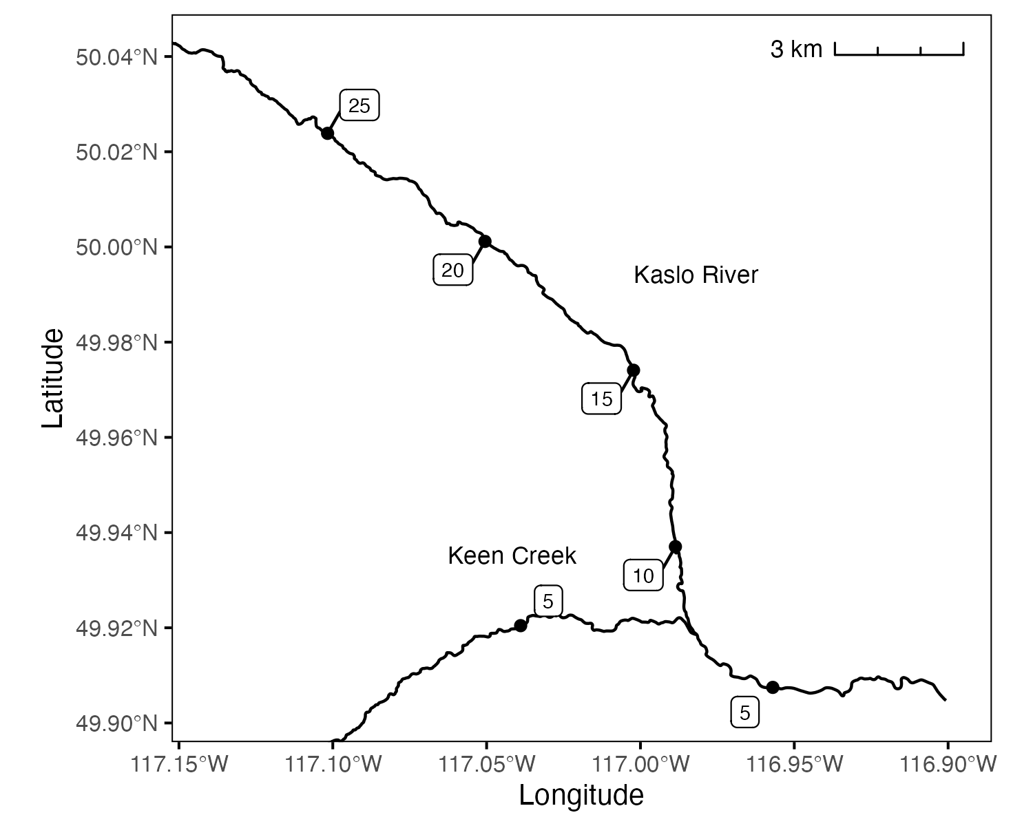
Figure 1. Spatial distribution of fish-bearing channel.
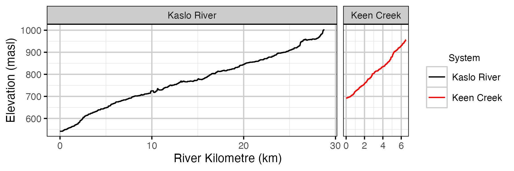
Figure 2. Channel elevation by river kilometre and system.
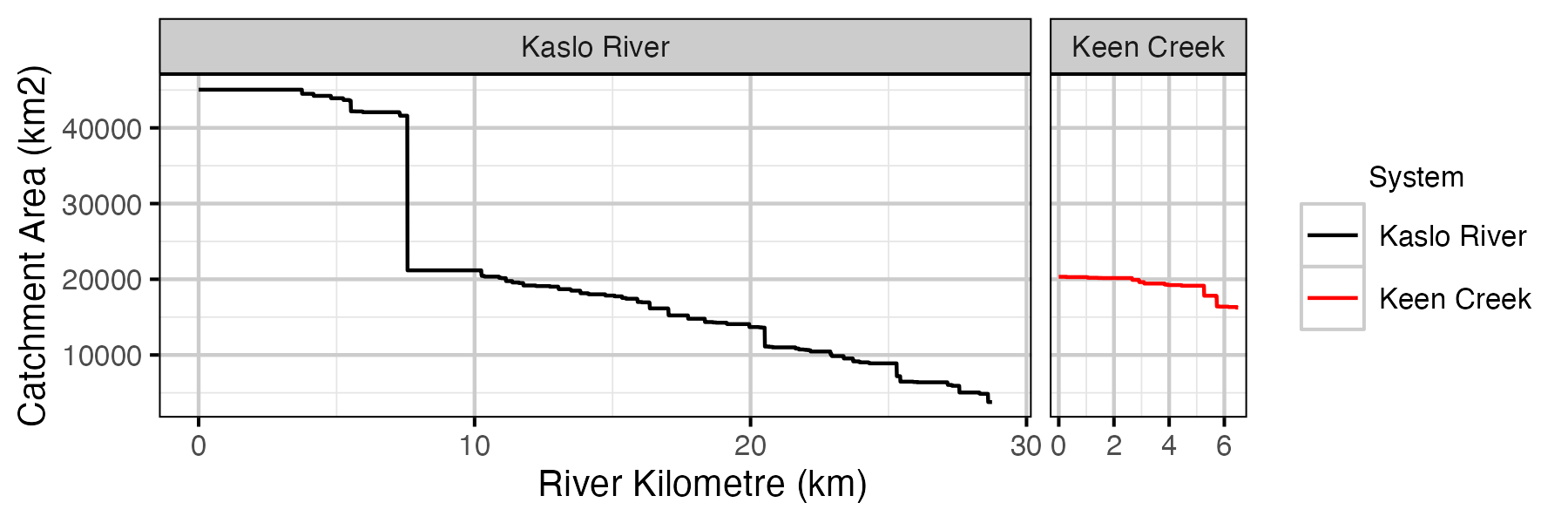
Figure 3. Catchment area by river kilometre and system.
Sites
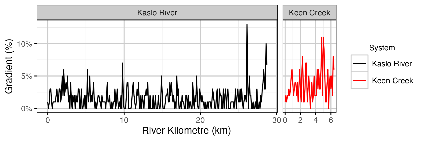
Figure 4. Site gradient by river kilometre and system.
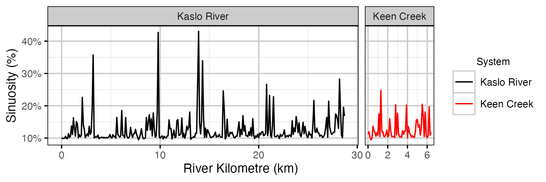
Figure 5. Site sinuosity by river kilometre and system.
Coverage
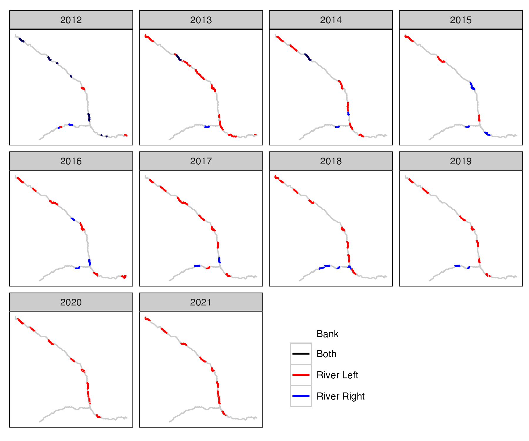
Figure 6. Snorkel count coverage by year and bank.
Length Correction
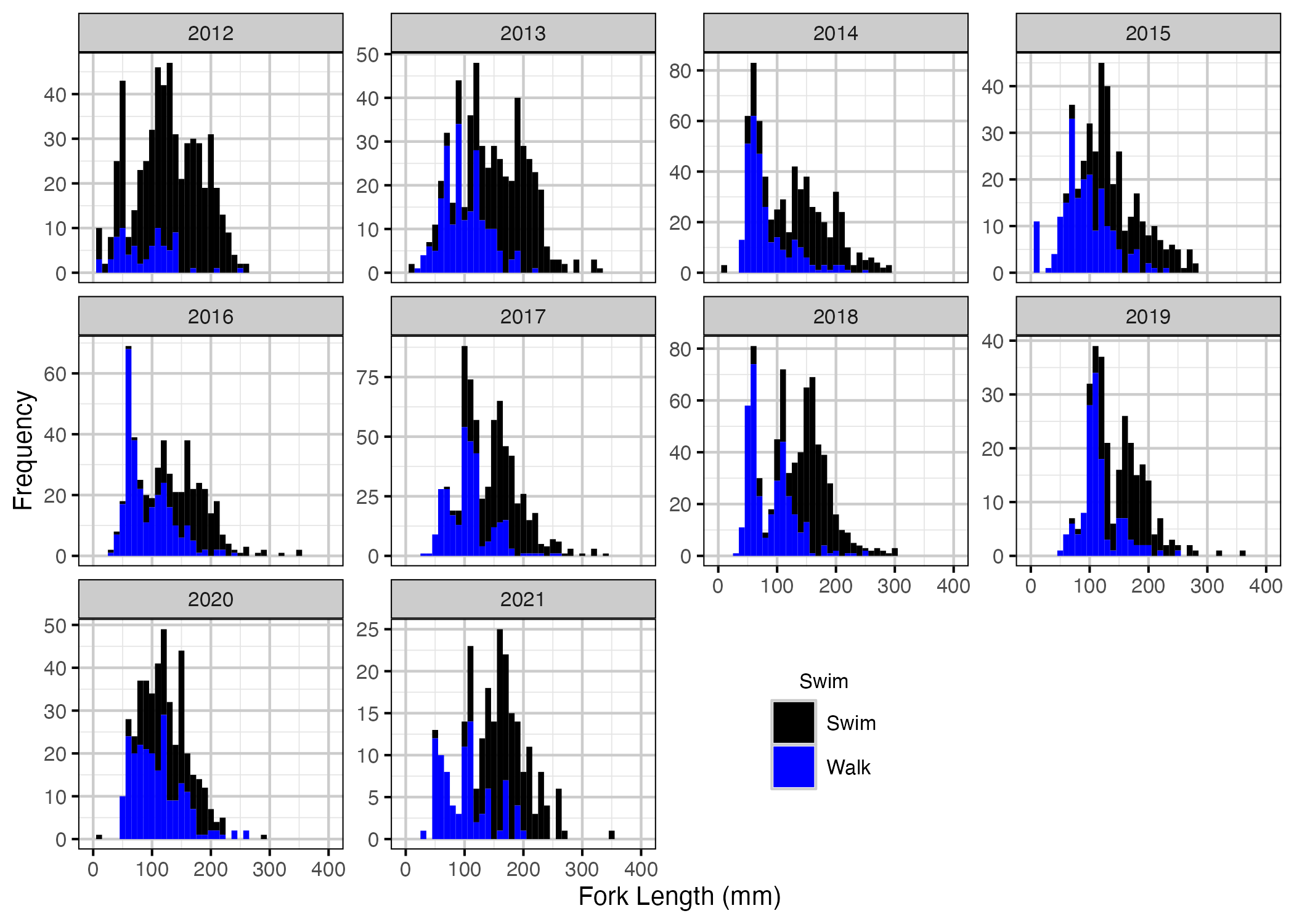
Figure 7. Corrected length-frequency histogram by year and observation type.
Fish
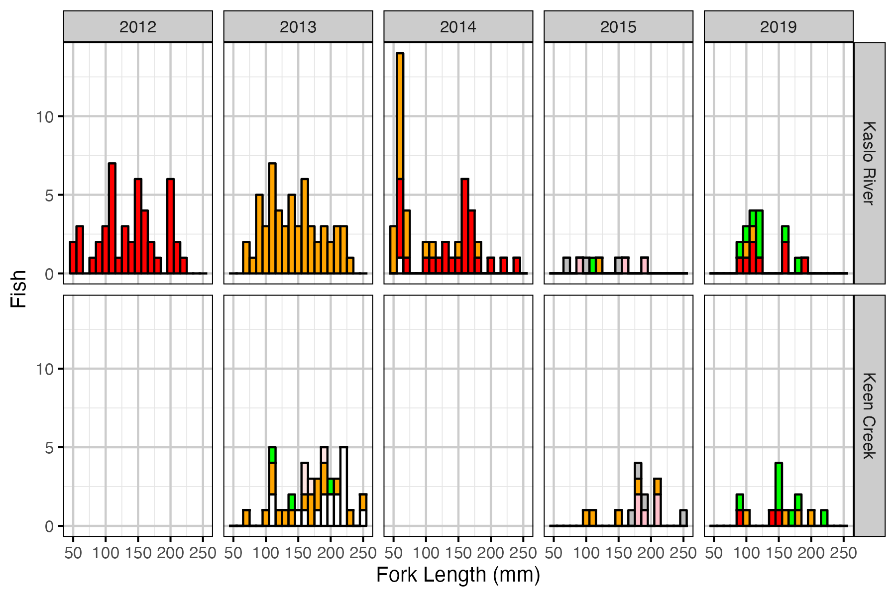
Figure 8. Length-frequency plot of marked Bull Trout by year and system.
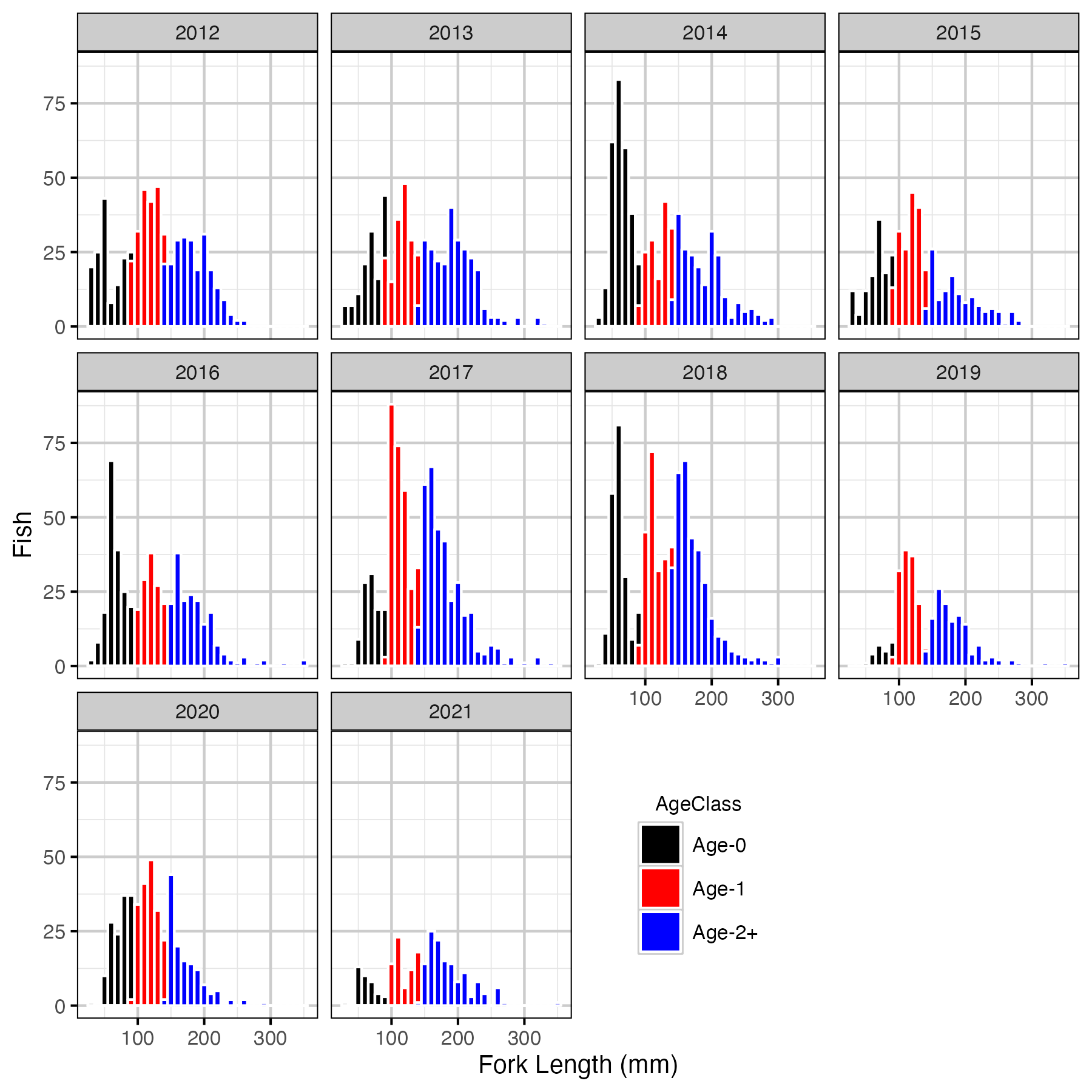
Figure 9. Length-frequency plot of observed Bull Trout by year.
Observer Efficiency
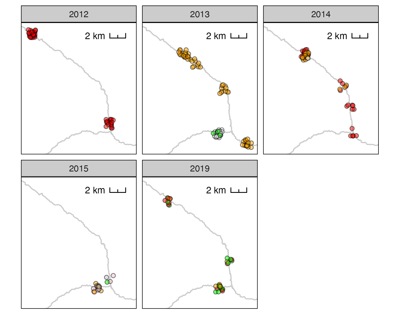
Figure 10. Distribution of marked juvenile Bull Trout by year and tag color.
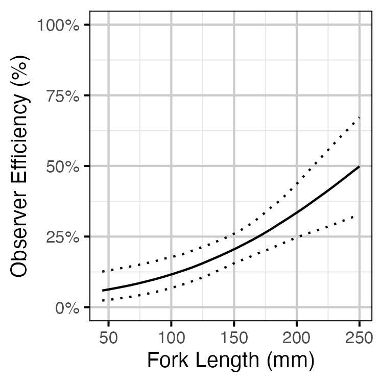
Figure 11. Estimated observer efficiency by fork length and system (with 95% CIs).
Lineal Density
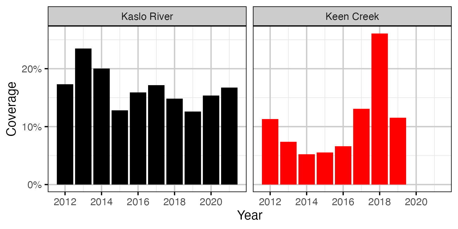
Figure 12. Percent coverage by year and system.
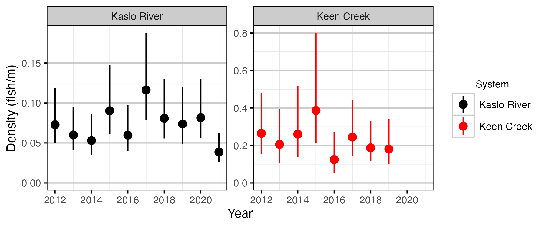
Figure 13. Estimated density by year and system (with 95% CIs).
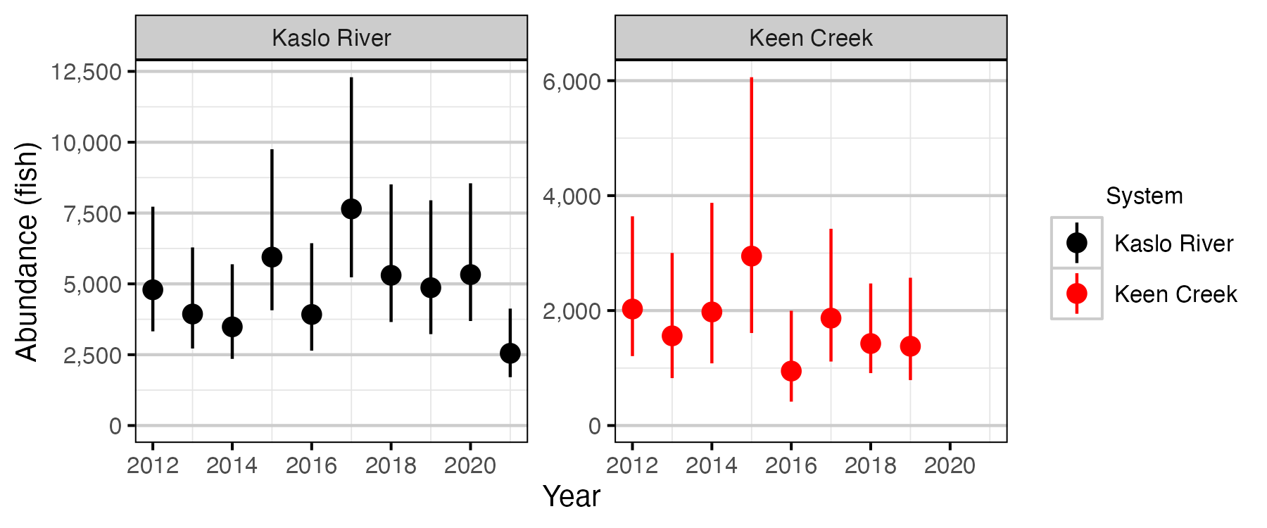
Figure 14. The estimated abundance by year and system (with 95% CIs).
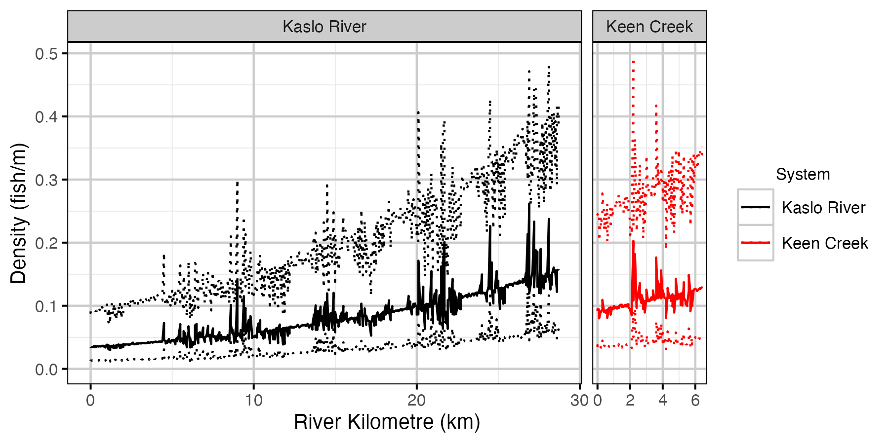
Figure 15. The estimated density by site and system (with 95% CIs).
Redds Stock-Recruiment
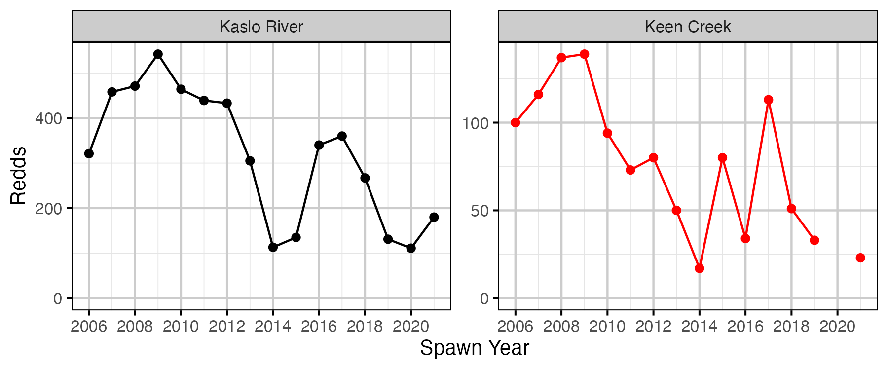
Figure 16. Complete redds by system and spawn year.
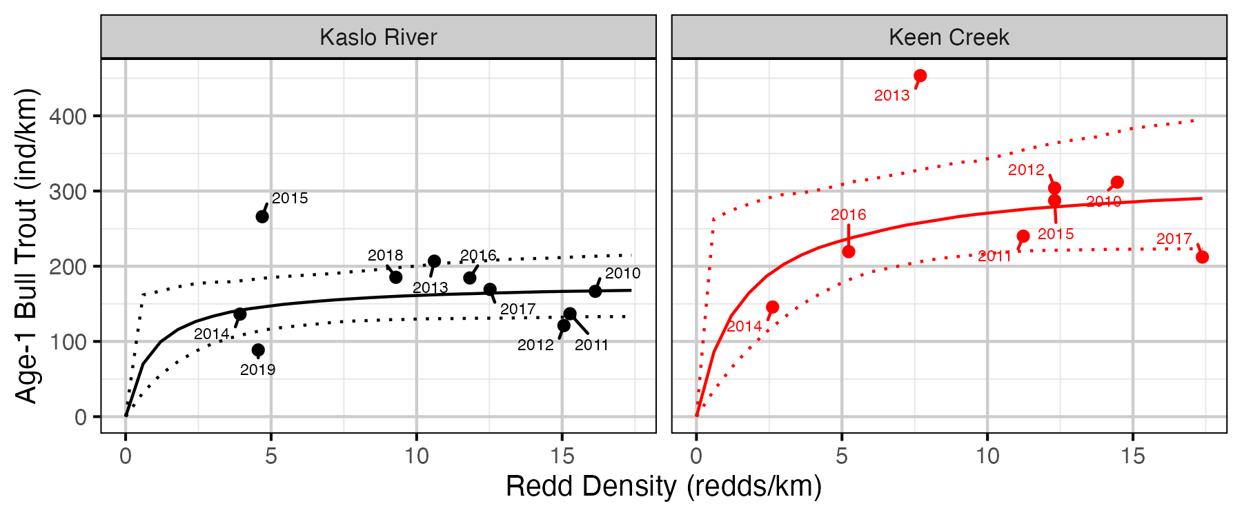
Figure 17. Estimated stock-recruitment relationship (with 95% CIs). The points are labelled by spawn year.
Condition
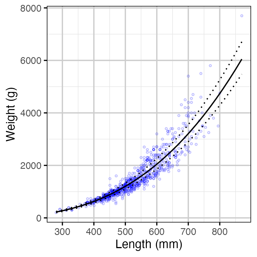
Figure 18. The weight-length relationship (with 95% CIs).
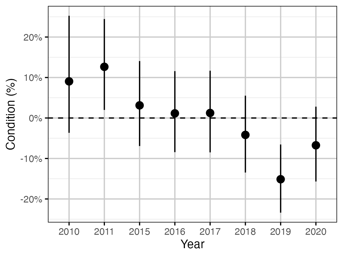
Figure 19. The percent change in the body condition for an average length fish relative to a typical year by year (with 95% CIs).
Fecundity
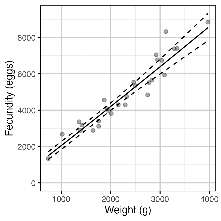
Figure 20. The predicted relationship between Fecundity and Weight for Bull Trout (with 95% CIs), data from Brunson (1952).
Spawner Length
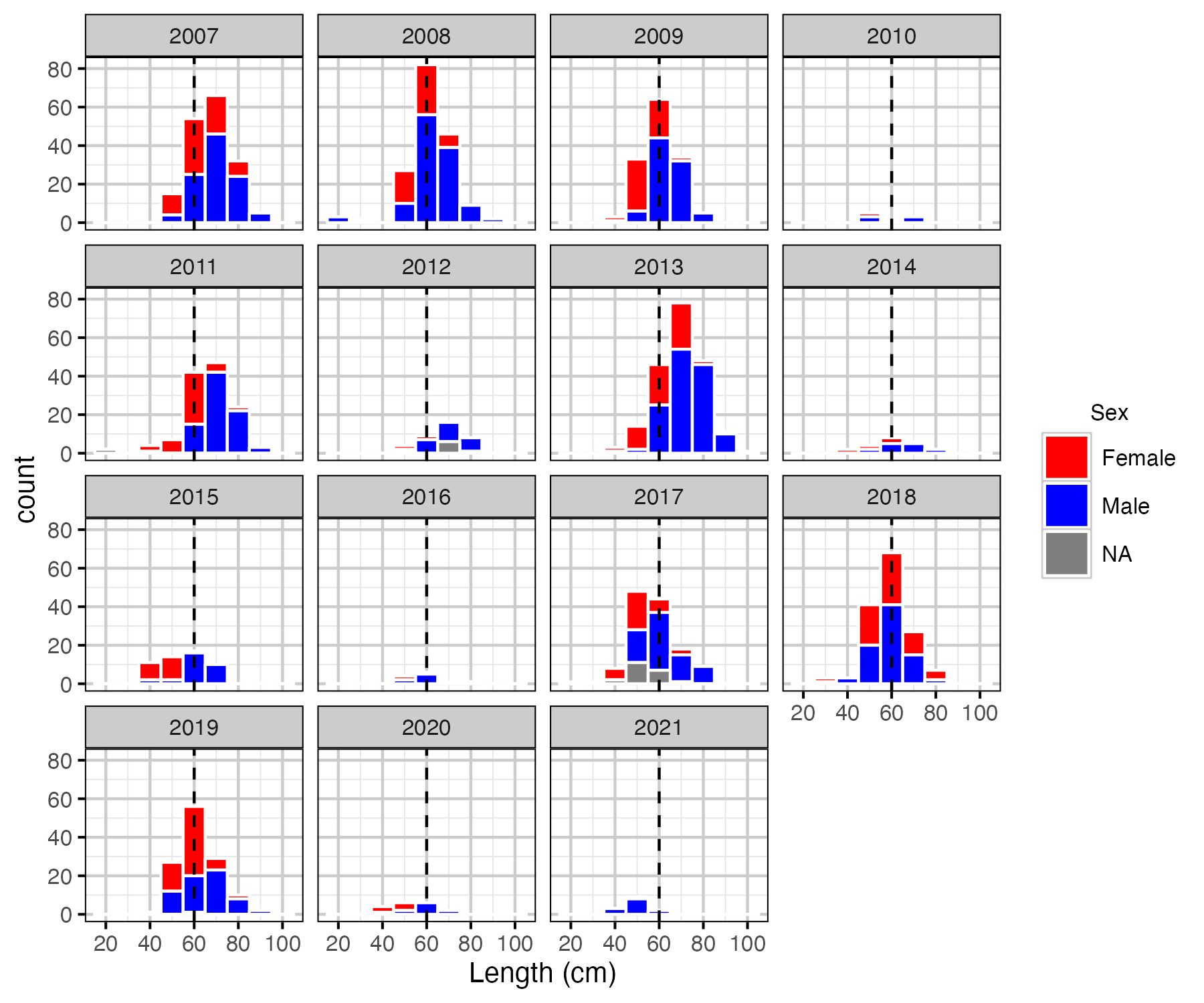
Figure 21. Length frequency of Bull Trout spawners by sex.
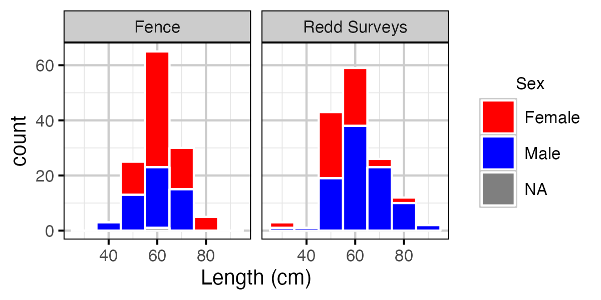
Figure 22. Length frequency of Bull Trout spawners by catch type in 2018 and 2019.
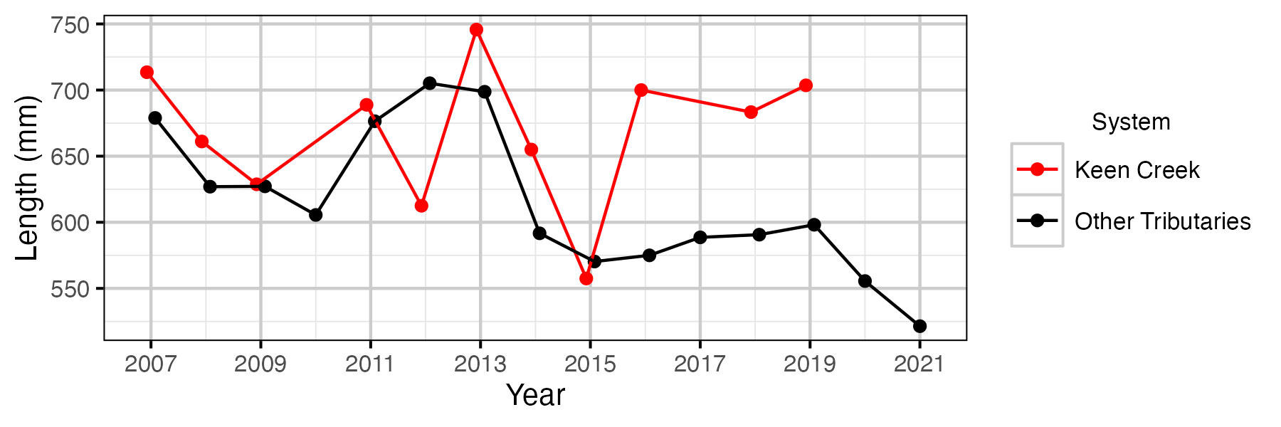
Figure 23. Average Length of Bull Trout spawners in Keen Creek compared to all other surveyed tributaries.
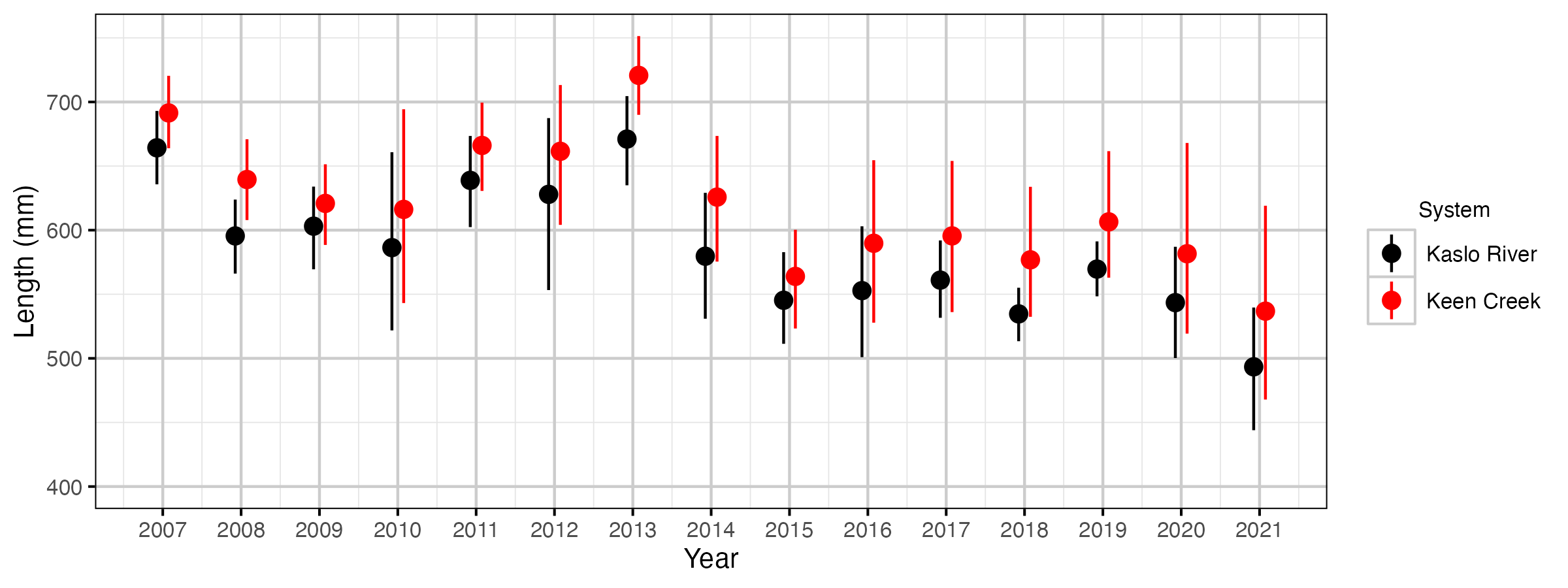
Figure 24. The expected length of female spawners by year for Kaslo River and Keen Creek (with 95% CIs).
Egg Deposition
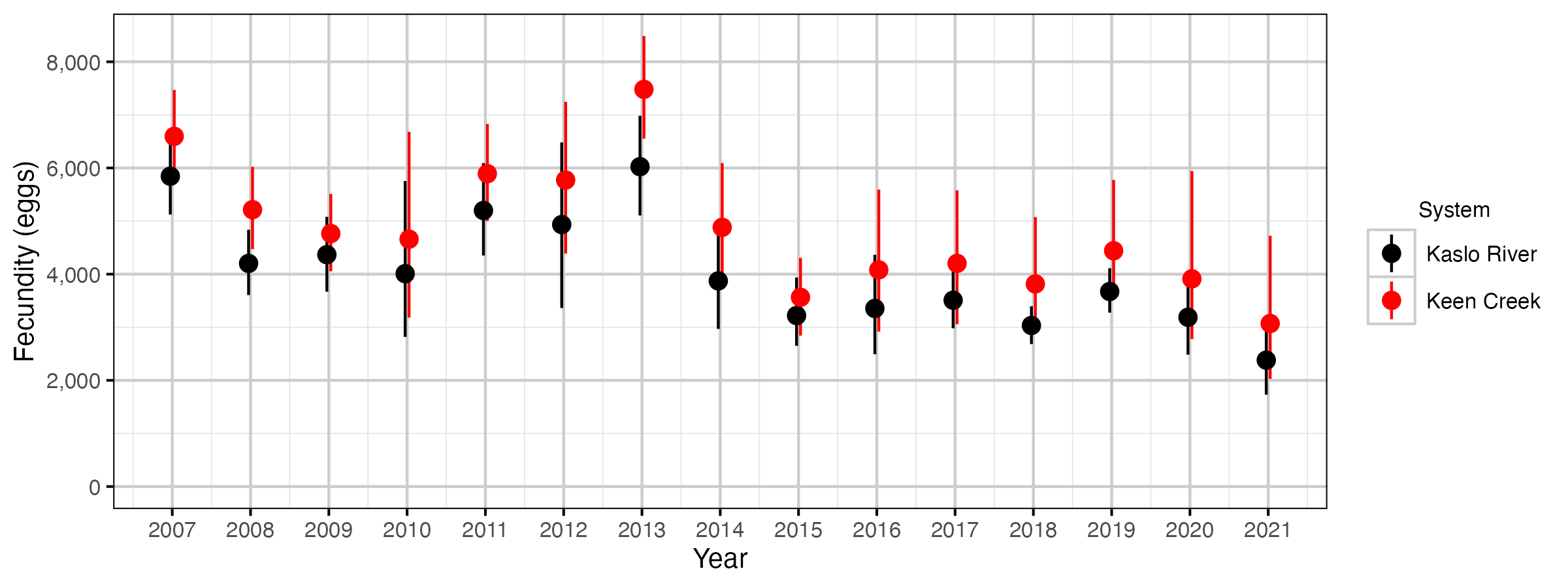
Figure 25. The estimated spawner fecundity by year uncorrected for condition (with 95% CIs).
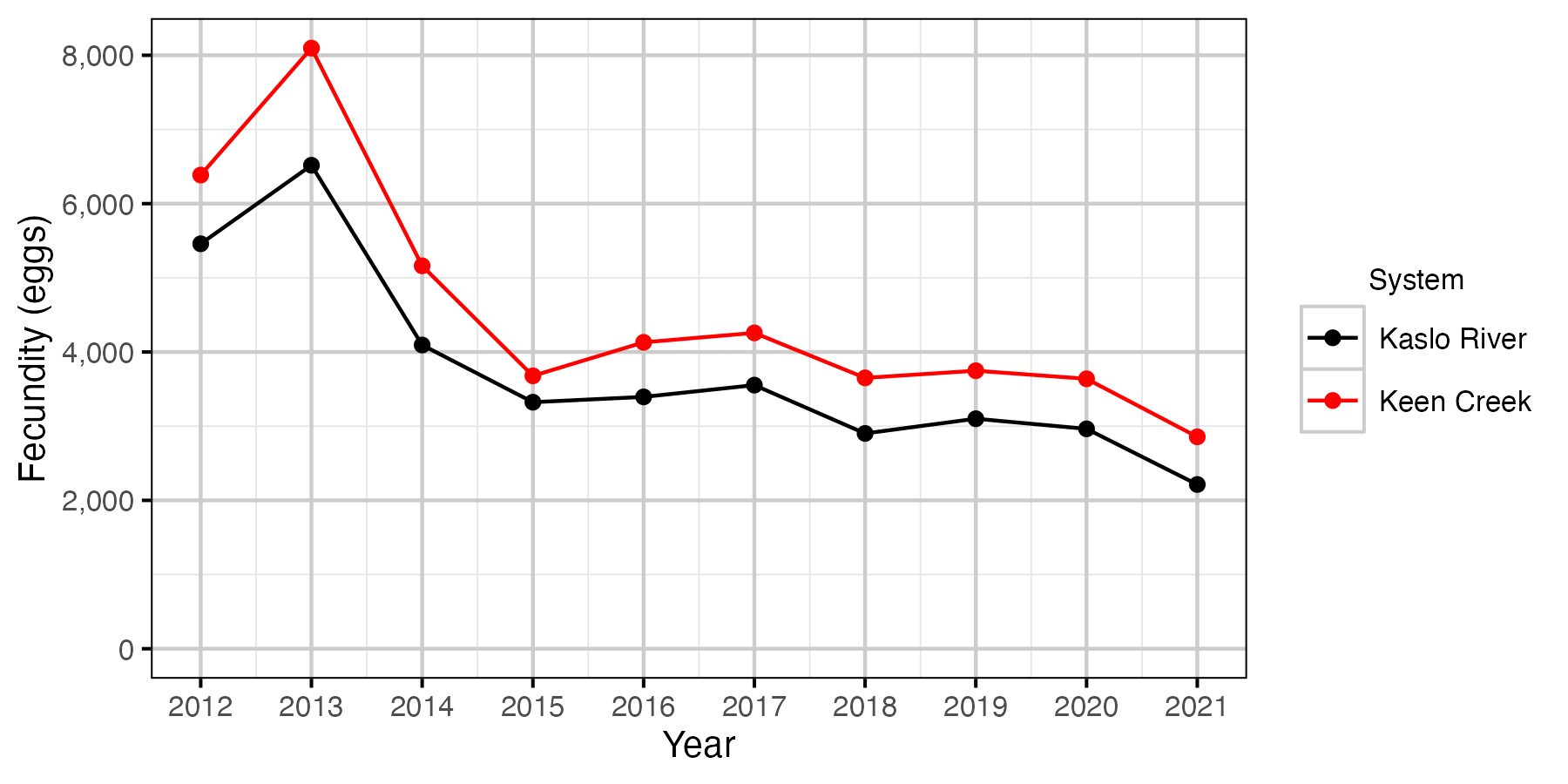
Figure 26. The estimated spawner fecundity by year corrected for condition.
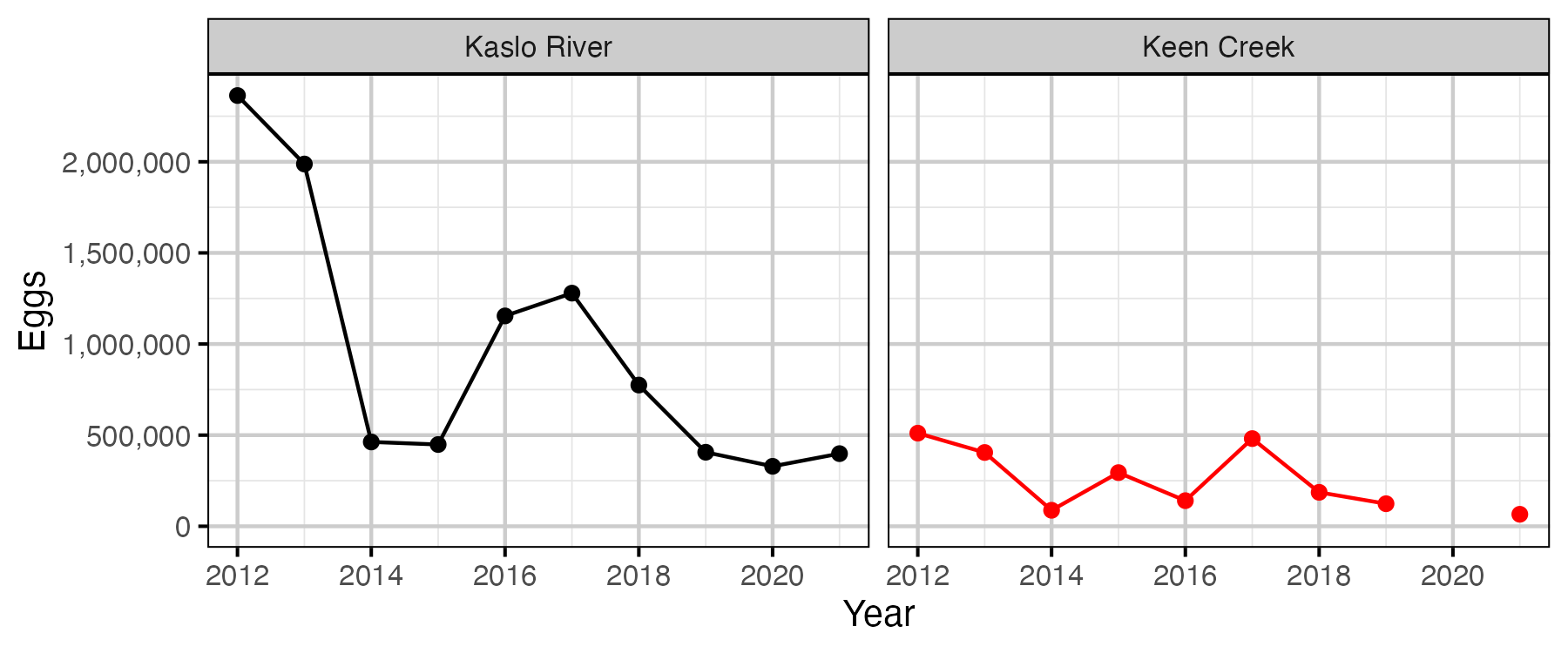
Figure 27. The estimated total egg deposition by system and year.
Eggs Stock-Recruiment
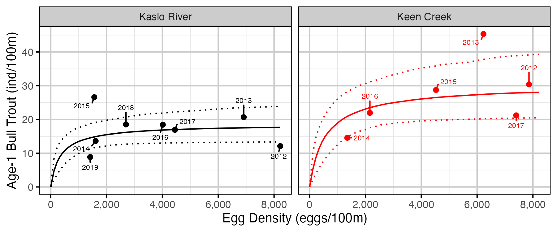
Figure 28. Estimated stock-recruitment relationship (with 95% CIs). The points are labelled by spawn year.
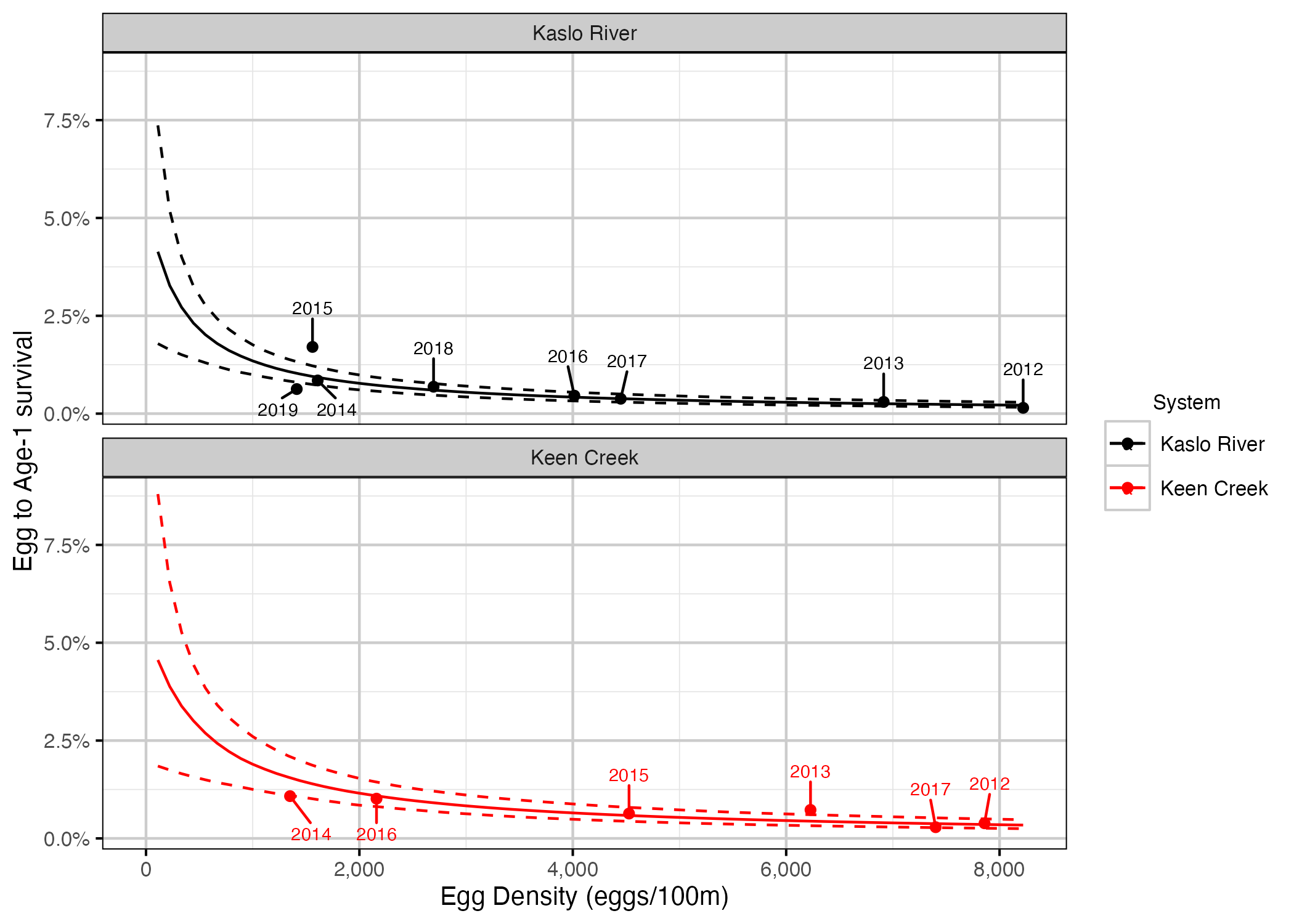
Figure 29. Predicted egg survival to age-1 by egg deposition (with 95% CRIs).
Conclusions
- Observer efficiency is approximately 17% for age-1 Bull Trout.
- Age-1 Bull Trout are relatively evenly distributed with respect to mesohabitat.
- Lineal densities of age-1 Bull Trout increase with river kilometre in both systems.
- The age-1 carrying capacity is estimated to be around 170 fish per km in Kaslo River and around 310 fish per km in Keen Creek.
Acknowledgements
The organisations and individuals whose contributions have made this analysis report possible include:
- Habitat Conservation Trust Foundation
- Ministry of Forest, Lands and Natural Resource Operations
- Greg Andrusak
- Emmanuel Abecia
- Ministry of Environment
- Jen Sarchuk
- BC Fish and Wildlife
- Trina Radford
- Stephan Himmer
- Gillian Sanders
- Jeff Berdusco
- Vicky Lipinski
- Jimmy Robbins
- Jason Bowers
- Seb Dalgarno