Horse Lake Exploitation Analysis 2021
The suggested citation for this analytic appendix is:
Thorley, J.L. & Pearson, A.D. (2022) Horse Lake Exploitation Analysis 2021. A Poisson Consulting Analytic Appendix. URL: https://www.poissonconsulting.ca/f/556371688.
Background
Horse Lake supports a recreational fishery for Lake Trout (Salvelinus namaycush). To estimate their natural and fishing mortality, individuals were caught by angling and tagged with acoustic transmitters and/or external reward tags. Acoustically tagged fish were detected by a series of seven receivers distributed through the lake as well as annual or biannual mobile detection surveys. The mobile detection survey was conducted by deploying receivers for approximately 10 minutes at 90 locations arranged on a 400 m x 400 m grid. The external reward tags included a phone number for anglers to report their recaptures. In 2009 and 2021, a summer profundal index netting (SPIN) survey was done on the lake.
All the data were provided by the Ministry of Forests, Lands and Natural Resource Operations (MFLNRO) Cariboo Region.
Data Preparation
The data were prepared for analysis using R version 4.2.0 (R Core Team 2021). Detections were aggregated daily, where for each transmitter the receiver with the most detections was chosen.
The Seasons were Winter (December - February), Spring (March - May), Summer (June - August) and Autumn (September - November).
For each mobile survey each detected fish was assigned a location corresponding to the centroid of its detection locations weighted by the detection rates. The mobile receiver deployment times were corrected by increasing or decreasing the deployment times for each receiver on each day by up to three minutes to maximize the number of detections within deployments. Mobile surveys conducted within 3 months of each other were combined into a single survey.
Statistical Analysis
Model parameters were estimated using Bayesian methods. The estimates were produced using JAGS (Plummer 2003) and STAN (Carpenter et al. 2017). For additional information on Bayesian estimation the reader is referred to McElreath (2016).
Unless stated otherwise, the Bayesian analyses used weakly informative normal and half-normal prior distributions (Gelman, Simpson, and Betancourt 2017). The posterior distributions were estimated from 1500 Markov Chain Monte Carlo (MCMC) samples thinned from the second halves of 3 chains (Kery and Schaub 2011, 38–40). Model convergence was confirmed by ensuring that the potential scale reduction factor \(\hat{R} \leq 1.05\) (Kery and Schaub 2011, 40) and the effective sample size (Brooks et al. 2011) \(\textrm{ESS} \geq 150\) for each of the monitored parameters (Kery and Schaub 2011, 61).
The parameters are summarised in terms of the point estimate, lower and upper 95% credible limits (CLs) and the surprisal s-value (Greenland 2019). The estimate is the median (50th percentile) of the MCMC samples while the 95% CLs are the 2.5th and 97.5th percentiles. The s-value can be considered a test of directionality. More specifically it indicates how surprising (in bits) it would be to discover that the true value of the parameter is in the opposite direction to the estimate. An s-value (Chow and Greenland 2019) is the Shannon transform (-log to base 2) of the corresponding p-value (Kery and Schaub 2011; Greenland and Poole 2013). A surprisal value of 4.3 bits, which is equivalent to a p-value of 0.05 indicates that the surprise would be equivalent to throwing 4.3 heads in a row. The condition that non-essential explanatory variables have s-values \(\geq\) 4.3 bits provides a useful model selection heuristic (Kery and Schaub 2011).
Model adequacy was assessed via posterior predictive checks (Kery and Schaub 2011). More specifically, the first four central moments (mean, variance, skewness and kurtosis) for the deviance residuals were compared to the expected values by simulating new residuals. In this context the s-value indicates how surprising each metric is given the estimated posterior probability distribution for the residual variation.
Where computationally practical, the sensitivity of the parameters to the choice of prior distributions was evaluated by increasing the standard deviations of all normal, half-normal and log-normal priors by an order of magnitude and then using \(\hat{R}\) to test whether the samples where drawn from the same posterior distribution (Thorley and Andrusak 2017).
The results are displayed graphically by plotting the modeled relationships between particular variables and the response(s) with the remaining variables held constant. In general, continuous and discrete fixed variables are held constant at their mean and first level values, respectively, while random variables are held constant at their typical values (expected values of the underlying hyperdistributions) (Kery and Schaub 2011, 77–82). When informative the influence of particular variables is expressed in terms of the effect size (i.e., percent or n-fold change in the response variable) with 95% credible intervals (CIs, Bradford, Korman, and Higgins 2005).
The analyses were implemented using R version 4.2.0
(R Core Team 2021) and the
mbr family of packages.
Model Descriptions
Condition
The expected weight, \(W\), of a fish of a given length, \(L\), was estimated from the data using an allometric mass-length model (He et al. 2008)
\[ W = \alpha L^\beta\]
Key assumptions of the condition model include:
- The prior distribution on the power term (\(\beta\)) is a normal distribution with a mean of 3.18 and a standard deviation of 0.19 (McDermid, Shuter, and Lester 2010).
- The weight varies by day of the year.
- The residual variation in weight is log-normally distributed.
Preliminary analysis indicated year as a random effect and capture method (angling vs SPIN) were not important predictors of condition.
Growth and Spawning
The growth curve and length at spawning for each ecotype were estimated from the length, scale age, and spawning data using an integrated model. The model consists of a biphasic Von Bertalanffy (von Bertalanffy 1938) growth curve and length at spawning model.
The Von Bertalanffy growth curve (von Bertalanffy 1938) for the small ecotype is
\[ L = L_{\infty_{1}} \cdot (1 - \exp(-k_1 \cdot A ))\]
where \(A\) is the scale age in years.
The large ecotype transitions to the second growth phase at the transitions age (\(A_T\)), where \(L_T\) is the transition length (mm)
\[ L_T = L_{\infty_{1}} \cdot (1 - \exp(-k_1 \cdot A_T )) \]
The Von Bertalanffy growth curve (von Bertalanffy 1938) in the second growth phase the large ecotype
\[ L = L_T + (L_{\infty_{2}} - L_T) \cdot (1 - \exp(-k_2 \cdot (A - A_T)))\]
The probability of spawning at length \(L\) is determined by
\[S = \frac{L^{S_p}}{L_s^{S_p} + L^{S_p}} \cdot es\]
Key assumptions of the model include:
- \(Ls\) varies by ecotype
- \(Es\) varies by ecotype
- Transition age, \(A_T\), varies randomly by fish
- The residual variation in length is log normally distributed.
The sensitivity analysis indicated that the estimate of bBigEs is
sensitive to the choice of prior. Increasing the standard deviation of
the prior by an order of magnitude increased the estimate from 1.71 (95%
CI 0.06 - 4.15) to 8.97 (95% CI 0.153 - 42.0).
Mobile
A fish was classified as being in the lake at the time of the survey if it was detected 1 or more times. A fish was classified as having moved if the weighted centriod had shifted more then 800 m since the previous survey.
Survival
The natural mortality and capture probability for individuals \(\geq\) 300 mm was estimated using a Bayesian individual state-space survival model (Thorley and Andrusak 2017) with three month intervals. The survival model incorporated natural mortality, fixed and mobile acoustic detection and movement, T-bar tag loss, recapture and reporting. Key assumptions of the survival model include:
- The natural mortality varies by season.
- The fishing mortality varies by year.
The survival model treats all recaptured fish as if they had been retained. Only individuals with a fork length (FL) \(\geq\) 300 mm that were tagged with an acoustic tag and/or $100 and $10 reward tags were included in the survival analysis.
Preliminary analysis indicated that there was not a clear difference between the natural mortality and fishing mortality rates for individuals \(\geq\) 500 mm.
Yield-Per-Recruit
The optimal capture rate (to maximize number of individuals harvested assuming 100% retention) was calculated using yield-per-recruit analysis (Walters and Martell 2004). A yield-per-recruit analysis was performed for the two different Lake Trout ecotypes separately and in combination. The \(Rk\) of 25 from Myers et al. (Myers, Bowen, and Barrowman 1999) was converted into the equivalent egg to age-1 survival of 0.025 based on the large ecotype life history
Model Templates
Condition
.model {
  bWeight ~ dnorm(-12, 2^-2)
  bWeightLength ~ dnorm(3.18, 0.19^-2)
  bDayte ~ dnorm(0, 2^-2)
  bDayte2 ~ dnorm(0, 2^-2)
  sWeight ~ dnorm(0, 1^-2) T(0,)
  for(i in 1:length(LogLength)) {
    eWeightLength[i] <- bWeightLength + bDayte * Dayte[i] + bDayte2 * Dayte[i]^2
    eWeight[i] <- bWeight + eWeightLength[i] * LogLength[i]
    Weight[i] ~ dlnorm(eWeight[i], sWeight^-2)
  }
Block 1. Condition model description.
Growth and Spawning
.model {
  bT0 <- 0

  bLInf1 ~ dnorm(6, 2^-2)
  bLInf2  ~ dnorm(7, 2^-2)
  bK1 ~ dnorm(0, 2^-2)
  bK2 ~ dnorm(0, 2^-2)
  bTransitionAge ~ dnorm(2, 1^-2)
  sTransitionAgeFish ~ dnorm(0, 2^-2) T(0,)
  bSmall ~ dnorm(0, 2^-2)
  sLength ~ dnorm(0, 2^-2) T(0, )

  Ls ~ dnorm(6, 2^-2)
  Sp ~ dnorm(20, 20^-2) T(0,)
  Es ~ dnorm(0, 2^-2)
  bBigLs ~ dnorm(0, 2^-2)
  bBigEs ~ dnorm(0, 2^-2)
  for (i in 1:nFishID) {
    bTransitionAgeFish[i] ~ dnorm(-sTransitionAgeFish^2/2, sTransitionAgeFish^-2)
  }
  for (i in 1:nObs) {
    logit(eSmall[i]) <- bSmall
    log(eLInf1[i]) <- bLInf1
    log(eLInf2[i]) <- bLInf2
    log(eK1[i]) <- bK1
    log(eK2[i]) <- bK2
    log(eLs[i]) <- Ls  + bBigLs * (1 - SmallEcotype[i])
    logit(eEs[i]) <- Es + bBigEs * (1 - SmallEcotype[i])
    eSpawning[i] <- ( (Length[i] ^ Sp) / (eLs[i]^Sp + Length[i]^Sp) ) * eEs[i]
    eSmallLength[i] <- eLInf1[i] * (1 - exp(-eK1[i] * (Age[i] - bT0)))

    log(eTransitionAge[i]) <- bTransitionAge + bTransitionAgeFish[FishID[i]]
    eTransitionLength[i] <- eLInf1[i] * (1 - exp(-eK1[i] * (eTransitionAge[i] - bT0)))
    eBigLength[i] <- eSmallLength[i] * step(eTransitionAge[i] - Age[i]) + step(Age[i] - eTransitionAge[i] - 0.01) * (eTransitionLength[i] + (eLInf2[i] - eTransitionLength[i]) * (1 - exp(-eK2[i] * (Age[i] - eTransitionAge[i]))))
    eLength[i] <-  eSmallLength[i] * SmallEcotype[i] + eBigLength[i] * (1 - SmallEcotype[i])
    Spawning[i] ~ dbin(eSpawning[i], 1)
    SmallEcotype[i] ~ dbin(eSmall[i], 1)
    Length[i] ~ dlnorm(log(eLength[i]), sLength^-2)
  }
Block 2. Growth model description.
Survival
.model{
  bMortality ~ dnorm(-3, 3^-2)
  bTagLoss ~ dbeta(1, 1)
  bMoved ~ dbeta(1, 1)
  bMobileDetected ~ dbeta(1, 1)
  bMobileMoved ~ dbeta(1, 1)
  bRecaptured ~ dnorm(0, 2^-2)
  bReported ~ dbeta(1, 1)
  bDetectedAlive ~ dbeta(1, 1)
  bDieNear ~ dbeta(1, 1)
  bDetectedDeadNear ~ dbeta(10, 1)
  bDetectedDeadFar ~ dbeta(1, 10)
  bMortalitySeason[1] <- 0
  for (i in 2:nSeason) {
    bMortalitySeason[i] ~ dnorm(0, 2^-2)
  }
  sRecapturedAnnual ~ dnorm(0, 2^-2) T(0,)
  for(i in 1:nAnnual) {
    bRecapturedAnnual[i] ~ dnorm(0, sRecapturedAnnual^-2)
  }

  for (i in 1:nCapture){
    eDetectedAlive[i] <- bDetectedAlive
    eDieNear[i] ~ dbern(bDieNear)
    eDetectedDeadNear[i] <- bDetectedDeadNear
    eDetectedDeadFar[i] <- bDetectedDeadFar
    eDetectedDead[i] <- eDieNear[i] * eDetectedDeadNear[i] + (1 - eDieNear[i]) * eDetectedDeadFar[i]
    logit(eMortality[i,PeriodCapture[i]]) <- bMortality + bMortalitySeason[Season[PeriodCapture[i]]]
    eTagLoss[i,PeriodCapture[i]] <- bTagLoss
    eDetected[i,PeriodCapture[i]] <- Alive[i,PeriodCapture[i]] * eDetectedAlive[i] + (1-Alive[i,PeriodCapture[i]]) * eDetectedDead[i]
    eMoved[i,PeriodCapture[i]] <- bMoved
    eMobileDetected[i,PeriodCapture[i]] <- bMobileDetected
    eMobileMoved[i,PeriodCapture[i]] <- bMobileMoved

    logit(eRecaptured[i,PeriodCapture[i]]) <- bRecaptured + bRecapturedAnnual[Annual[PeriodCapture[i]]]
    eReported[i,PeriodCapture[i]] <- bReported
    InLake[i,PeriodCapture[i]] <- 1
    Alive[i,PeriodCapture[i]] ~ dbern(1-eMortality[i,PeriodCapture[i]])
    TBarTag100[i,PeriodCapture[i]] ~ dbern(1-eTagLoss[i,PeriodCapture[i]])
    TBarTag10[i,PeriodCapture[i]] ~ dbern(1-eTagLoss[i,PeriodCapture[i]])
    Detected[i,PeriodCapture[i]] ~ dbern(Monitored[i,PeriodCapture[i]] * eDetected[i,PeriodCapture[i]])
    Moved[i,PeriodCapture[i]] ~ dbern(Alive[i,PeriodCapture[i]] * Monitored[i,PeriodCapture[i]] * eMoved[i,PeriodCapture[i]])
    MobileDetected[i,PeriodCapture[i]] ~ dbern(Monitored[i,PeriodCapture[i]] * eMobileDetected[i,PeriodCapture[i]] * MobileSurvey[i,PeriodCapture[i]])
    MobileMoved[i,PeriodCapture[i]] ~ dbern(Alive[i,PeriodCapture[i]] * MobileDetected[i,PeriodCapture[i]] * eMobileMoved[i,PeriodCapture[i]])
    Recaptured[i,PeriodCapture[i]] ~ dbern(Alive[i,PeriodCapture[i]] * eRecaptured[i,PeriodCapture[i]])
    Reported[i,PeriodCapture[i]] ~ dbern(Recaptured[i,PeriodCapture[i]] * eReported[i,PeriodCapture[i]] * step(TBarTag100[i,PeriodCapture[i]] + TBarTag10[i,PeriodCapture[i]] - 1))
  for(j in (PeriodCapture[i]+1):nPeriod) {
    logit(eMortality[i,j]) <- bMortality + bMortalitySeason[Season[j]]
    eTagLoss[i,j] <- bTagLoss

    eDetected[i,j] <- Alive[i,j] * eDetectedAlive[i] + (1-Alive[i,j]) * eDetectedDead[i]
    eMoved[i,j] <- bMoved
    eMobileDetected[i,j] <- bMobileDetected
    eMobileMoved[i,j] <- bMobileMoved
    logit(eRecaptured[i,j]) <- bRecaptured + bRecapturedAnnual[Annual[j]]
    eReported[i,j] <- bReported

    InLake[i,j] ~ dbern(InLake[i,j-1] * (1-Recaptured[i,j-1]))
    Alive[i,j] ~ dbern(Alive[i,j-1] * (1-Recaptured[i,j-1]) * (1-eMortality[i,j-1]))
    TBarTag100[i,j] ~ dbern(TBarTag100[i,j-1] * (1-Recaptured[i,j-1]) * (1-eTagLoss[i,j]))
    TBarTag10[i,j] ~ dbern(TBarTag10[i,j-1] * (1-Recaptured[i,j-1]) * (1-eTagLoss[i,j]))
    Detected[i,j] ~ dbern(InLake[i,j] * Monitored[i,j] * eDetected[i,j])
    Moved[i,j] ~ dbern(Alive[i,j] * Monitored[i,j] * eMoved[i,j])
    MobileDetected[i,j] ~ dbern(InLake[i,j] * Monitored[i,j] * eMobileDetected[i,j] * MobileSurvey[i,j])
    MobileMoved[i,j] ~ dbern(Alive[i,j] * MobileDetected[i,j] * eMobileMoved[i,j])
    Recaptured[i,j] ~ dbern(Alive[i,j] * eRecaptured[i,j])
    Reported[i,j] ~ dbern(Recaptured[i,j] * eReported[i,j] * step(TBarTag100[i,j] + TBarTag10[i,j] - 1))}}
  }
Block 3. Survival model description.
Results
Tables
Condition
Table 1. Parameter descriptions.
| Parameter | Description |
|---|---|
bDayte |
Effect of Dayte on eWeight |
bDayte2 |
Effect of Dayte on bDayte |
bWeight |
Intercept of eWeight |
bWeightLength |
Effect of Length on bWeight |
eWeight |
Log expected Weight |
LogLength |
Log-transformed and centered fork length (mm) |
sWeight |
Standard deviation of residual variation in eWeight |
Weight |
Mass (kg) |
Table 2. Model coefficients.
| term | estimate | lower | upper | svalue |
|---|---|---|---|---|
| bDayte | 0.0021305 | -0.0021943 | 0.0063186 | 1.526569 |
| bDayte2 | 0.0047673 | 0.0016263 | 0.0081273 | 7.744353 |
| bWeight | -11.8283665 | -12.0569461 | -11.6264196 | 10.551708 |
| bWeightLength | 3.0924035 | 3.0363606 | 3.1540408 | 10.551708 |
| sWeight | 0.1329065 | 0.1232997 | 0.1438934 | 10.551708 |
Table 3. Model convergence.
| n | K | nchains | niters | nthin | ess | rhat | converged |
|---|---|---|---|---|---|---|---|
| 328 | 5 | 3 | 500 | 100 | 238 | 1.018 | TRUE |
Table 4. Model posterior predictive checks.
| moment | observed | median | lower | upper | svalue |
|---|---|---|---|---|---|
| zeros | NA | NA | NA | NA | NA |
| mean | -0.0030955 | 0.0023552 | -0.1051842 | 0.1087159 | 0.1139562 |
| variance | 0.9878805 | 0.9961087 | 0.8550009 | 1.1479161 | 0.1223015 |
| skewness | 0.3855342 | 0.0032236 | -0.2593469 | 0.2666003 | 8.2297802 |
| kurtosis | 1.4622530 | -0.0483514 | -0.4643365 | 0.5921388 | 10.5517083 |
Table 5. Model sensitivity.
| n | K | nchains | niters | rhat_1 | rhat_2 | rhat_all | converged |
|---|---|---|---|---|---|---|---|
| 328 | 5 | 3 | 500 | 1.018 | 1.01 | 1.027 | TRUE |
Growth and Spawning
Table 6. Parameter descriptions.
| Parameter | Description |
|---|---|
Age[i] |
Scale age at capture (yr) |
bBigEs |
Effect of large ecotype on Es |
bBigLs |
Effect of the large ecotype on Ls |
bK1 |
Log growth coefficient (mm/yr) during the first phase of growth |
bK2 |
Log growth coefficient (mm/yr) during the second phase of growth |
bLInf1 |
Log mean maximum length (mm) for first phase of growth |
bLInf2 |
Log mean maximum length (mm) for second phase of growth |
bSmall |
Log odds probability a fish has the small ecotype life history |
bT0 |
Age at zero length (yr) |
bTransitionAge |
Log age large ecotype fish transition to the second phase of growth |
Es |
Log odds annual probability of a mature fish spawning |
Length[i] |
Fork length at capture (mm) |
Ls |
Log length (mm) at which 50% mature |
sLength |
SD of residual variation in log Length |
Sp |
Spawning maturity power |
sTransitionAgeFish |
SD of residual variation in bTransitionAge |
Table 7. Model coefficients.
| term | estimate | lower | upper | svalue |
|---|---|---|---|---|
| Es | 1.0417397 | 0.4332466 | 1.9217454 | 8.966746 |
| Ls | 5.8984343 | 5.8679668 | 5.9322331 | 10.551708 |
| Sp | 32.6076121 | 19.4434765 | 51.3165939 | 10.551708 |
| bBigEs | 1.7078693 | 0.0615577 | 4.1539655 | 4.529340 |
| bBigLs | 0.3840923 | 0.3280289 | 0.4364732 | 10.551708 |
| bK1 | -1.5827652 | -1.6674660 | -1.5043176 | 10.551708 |
| bK2 | -2.7336179 | -4.0508276 | -1.8753437 | 10.551708 |
| bLInf1 | 6.0636044 | 6.0357079 | 6.0972590 | 10.551708 |
| bLInf2 | 6.9929639 | 6.7086035 | 7.8147962 | 10.551708 |
| bSmall | 0.4894604 | 0.0674820 | 0.9907110 | 5.422425 |
| bTransitionAge | 2.3896863 | 2.1462053 | 2.5681527 | 10.551708 |
| sLength | 0.0943615 | 0.0856521 | 0.1044038 | 10.551708 |
| sTransitionAgeFish | 0.3083315 | 0.1827292 | 0.6609970 | 10.551708 |
Table 8. Model convergence.
| n | K | nchains | niters | nthin | ess | rhat | converged |
|---|---|---|---|---|---|---|---|
| 287 | 13 | 3 | 500 | 120 | 380 | 1.008 | TRUE |
Table 9. Model posterior predictive checks.
| moment | observed | median | lower | upper | svalue |
|---|---|---|---|---|---|
| zeros | NA | NA | NA | NA | NA |
| mean | 0.1679682 | 0.0008721 | -0.2318308 | 0.2543731 | 2.4695592 |
| variance | 0.5074504 | 0.9870565 | 0.6930691 | 1.3776126 | 10.5517083 |
| skewness | 0.6571235 | -0.0191969 | -0.5672586 | 0.5755957 | 5.5975120 |
| kurtosis | 0.0750760 | -0.1932583 | -0.8494504 | 1.3502731 | 0.7427441 |
Table 10. Model sensitivity.
| n | K | nchains | niters | rhat_1 | rhat_2 | rhat_all | converged |
|---|---|---|---|---|---|---|---|
| 287 | 13 | 3 | 500 | 1.008 | 4.246 | 4.985 | FALSE |
Survival
Table 11. Parameter descriptions.
| Parameter | Description |
|---|---|
bDetected |
Probability of detection (by the fixed receivers) if inlake in a three month period |
bDetectedAlive |
Probability of being detected if alive |
bDetectedDeadFar |
Probability of being dead and being far from a fixed receiver |
bDetectedDeadNear |
Probability of being dead and being near a fixed receiver |
bDieNear |
Probability of being dead |
bMobileDetected |
Probability of detection (by a mobile survey) if inlake |
bMobileMoved |
Probability of being detected moving between (mobile) surveys |
bMortality |
Log odds probability of dying of natural causes in a three month period |
bMortalitySeason[i] |
Effect of ith season on bMortality |
bMoved |
Probability of being detected (by the fixed receivers) moving between sections if alive in a three month period |
bRecaptured |
Log odds probability of being recaptured if alive for fish in a three month period |
bRecapturedAnnual[i] |
Effect of ith year on bRecaptured |
bReported |
Probability of being reported if recaptured with one or more T-bar tags |
bTagLoss |
Probability of loss for a single T-bar tag in a three month period |
Table 12. Model coefficients.
| term | estimate | lower | upper | svalue |
|---|---|---|---|---|
| bDetectedAlive | 0.9855262 | 0.9794279 | 0.9902420 | 10.551708 |
| bDetectedDeadFar | 0.0104891 | 0.0004314 | 0.0454864 | 10.551708 |
| bDetectedDeadNear | 0.9504023 | 0.7863229 | 0.9978776 | 10.551708 |
| bDieNear | 0.1396129 | 0.0155440 | 0.3270343 | 10.551708 |
| bMobileDetected | 0.7916780 | 0.7630119 | 0.8171409 | 10.551708 |
| bMobileMoved | 0.2941965 | 0.2518904 | 0.3382537 | 10.551708 |
| bMortality | -3.8324704 | -4.6460152 | -3.1975984 | 10.551708 |
| bMortalitySeason[2] | -0.0123237 | -0.8856008 | 0.9246724 | 0.025209 |
| bMortalitySeason[3] | 0.3628897 | -0.4733676 | 1.3007538 | 1.301410 |
| bMortalitySeason[4] | -0.1916711 | -1.2406876 | 0.9331460 | 0.462920 |
| bMoved | 0.8971551 | 0.8820556 | 0.9112939 | 10.551708 |
| bRecaptured | -3.9955795 | -4.8197073 | -2.8764164 | 10.551708 |
| bReported | 0.9937975 | 0.9685624 | 0.9997632 | 10.551708 |
| bTagLoss | 0.0047840 | 0.0021852 | 0.0090422 | 10.551708 |
| sRecapturedAnnual | 0.7245979 | 0.2647079 | 2.3038327 | 10.551708 |
Table 13. Model convergence.
| n | K | nchains | niters | nthin | ess | rhat | converged |
|---|---|---|---|---|---|---|---|
| 10336 | 15 | 3 | 500 | 150 | 226 | 1.013 | TRUE |
Yield-per-Recruit
Table 14. Summary of parameters in yield-per-recruit model.
| Parameter | Ecotype | Estimate | Description | Source |
|---|---|---|---|---|
| tmax | Small | 3.00e+01 | The maximum age (yr). | Professional Judgement |
| k | Small | 2.05e-01 | The VB growth coefficient (yr-1). | Current Study |
| Linf | Small | 4.30e+01 | The VB mean maximum length (cm). | Current Study |
| t0 | Small | 0.00e+00 | The (theoretical) age at zero length (yr). | Default |
| k2 | Large | 6.50e-02 | The VB growth coefficient after length L2 (yr-1). | Current Study |
| Linf2 | Large | 1.09e+02 | The VB mean maximum length after length L2 (cm). | Current Study |
| L2 | Large | -1.09e+01 | The length (or age if negative) at which growth switches from the | |
| first to second phase (cm or yr). | Current Study | |||
| Wb | Small | 3.09e+00 | The weight (as a function of length) scaling exponent. | Current Study |
| Ls | Large | 5.35e+01 | The length (or age if negative) at which 50 % mature (cm or yr). | Current Study |
| Ls | Small | 3.64e+01 | The length (or age if negative) at which 50 % mature (cm or yr). | Current Study |
| Sp | Small | 3.26e+01 | The maturity (as a function of length) power. | Current Study |
| es | Large | 9.39e-01 | The annual probability of a mature fish spawning. | Current Study |
| es | Small | 7.39e-01 | The annual probability of a mature fish spawning. | Current Study |
| Sm | Small | 0.00e+00 | The spawning mortality probability. | Default |
| fb | Small | 1.00e+00 | The fecundity (as a function of weight) scaling exponent. | Default |
| tR | Small | 1.00e+00 | The age from which survival is density-independent (yr). | Default |
| BH | Small | 1.00e+00 | Recruitment follows a Beverton-Holt (1) or Ricker (0) relationship. | Default |
| Rk | Small | 2.50e-02 | The lifetime spawners per spawner at low density (or the egg to tR survival if between 0 and 1). | Myers et al. 1999 |
| n | Small | 1.50e-01 | The annual interval natural mortality rate from age tR. | Default |
| nL | Small | 8.93e-02 | The annual interval natural mortality rate from length Ln. | Current Study |
| Ln | Small | 1.00e+03 | The length (or age if negative) at which the natural mortality | |
| rate switches from n to nL (cm or yr). | Default | |||
| Lv | Small | 3.50e+01 | The length (or age if negative) at which 50 % vulnerable to harvest | |
| (cm or yr). | Professional Judgement | |||
| Vp | Small | 2.50e+01 | The vulnerability to harvest (as a function of length) power. | Professional Judgement |
| Llo | Small | 0.00e+00 | The lower harvest slot length (cm). | Default |
| Lup | Small | 1.00e+03 | The upper harvest slot length (cm). | Default |
| Nc | Small | 0.00e+00 | The slot limits non-compliance probability. | Default |
| pi | Small | 6.85e-02 | The annual capture probability. | Current Study |
| rho | Small | 0.00e+00 | The release probability. | Default |
| Hm | Small | 0.00e+00 | The hooking mortality probability. | Default |
| Rmax | Small | 1.00e+00 | The number of recruits at the carrying capacity (ind). | Default |
| Wa | Small | 7.29e-03 | The (extrapolated) weight of a 1 cm individual (g). | Current Study |
| fa | Small | 1.00e+00 | The (theoretical) fecundity of a 1 g female (eggs). | Default |
| q | Small | 1.00e-01 | The catchability (annual probability of capture) for a unit of | |
| effort. | Default | |||
| RPR | Small | 6.20e-01 | The relative proportion of recruits that are of the ecotype. | Current Study |
Table 15. Lake Trout small ecotype yield-per-recruit calculations including the capture probability (pi), exploitation rate (u) and average age, length and weight of fish harvested.
| Type | pi | u | Yield | Age | Length | Weight | Effort |
|---|---|---|---|---|---|---|---|
| actual | 0.0685367 | 0.0685367 | 0.0784155 | 12.19239 | 38.39900 | 588.1968 | 0.6738626 |
| optimal | 0.2505139 | 0.2505139 | 0.1325517 | 10.19728 | 37.05659 | 525.9638 | 2.7369601 |
Table 16. Lake Trout large ecotype yield-per-recruit calculations including the capture probability (pi), exploitation rate (u) and average age, length and weight of fish harvested.
| Type | pi | u | Yield | Age | Length | Weight | Effort |
|---|---|---|---|---|---|---|---|
| actual | 0.0685367 | 0.0685367 | 0.0855306 | 12.18889 | 45.24860 | 1218.2181 | 0.6738626 |
| optimal | 0.1527720 | 0.1527720 | 0.1198807 | 11.03421 | 41.84701 | 900.0437 | 1.5735068 |
Table 17. Lake Trout (both ecotypes) yield-per-recruit calculations including the capture probability (pi), exploitation rate (u) and average age, length and weight of fish harvested.
| Type | pi | u | Yield | Age | Length | Weight | Effort |
|---|---|---|---|---|---|---|---|
| actual | 0.0685367 | 0.0685367 | 0.0819684 | 12.19105 | 41.01773 | 829.0659 | 0.6738626 |
| optimal | 0.1892544 | 0.1892544 | 0.1231963 | 10.67654 | 38.71312 | 645.1004 | 1.9912675 |
Table 18. Lake Trout (both ecotypes) stock-recruitment calculations including the capture probability (pi), exploitation rate (u) the relative number of eggs, recruits and spawners, and the average fecundity.
| Type | pi | u | Eggs | Recruits | Spawners | Fecundity |
|---|---|---|---|---|---|---|
| unfished | 0.0000000 | 0.0000000 | 578.47634 | 0.9353249 | 0.8752482 | 1321.8567 |
| actual | 0.0685367 | 0.0685367 | 284.83842 | 0.8768619 | 0.5375649 | 1059.7360 |
| optimal | 0.1892544 | 0.1892544 | 93.10331 | 0.6994816 | 0.2425527 | 767.6954 |
Figures
Captures
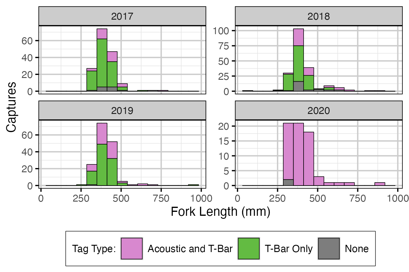
Figure 1. Lake Trout captures by fork length, year and tag type.
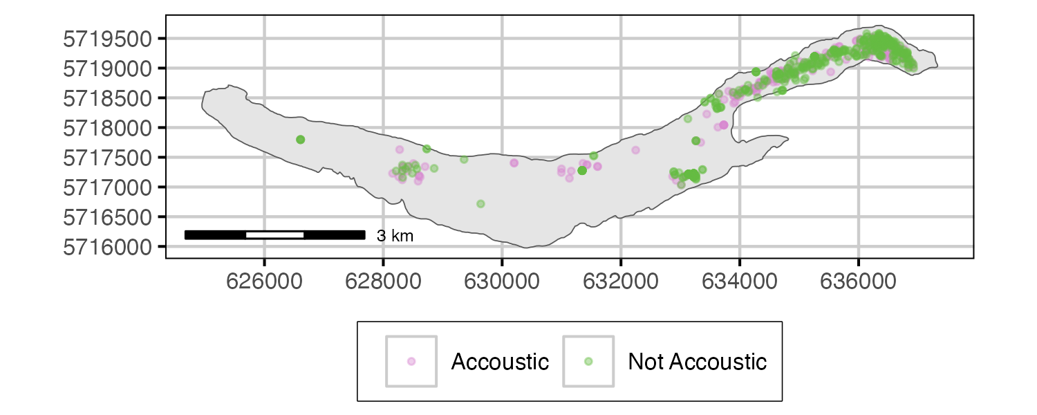
Figure 2. Lake Trout capture location by tagging.
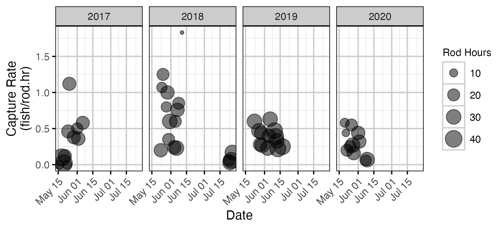
Figure 3. Angling capture rate for Lake Trout and date for fish with fork length > 300 mm.
Length Distribution
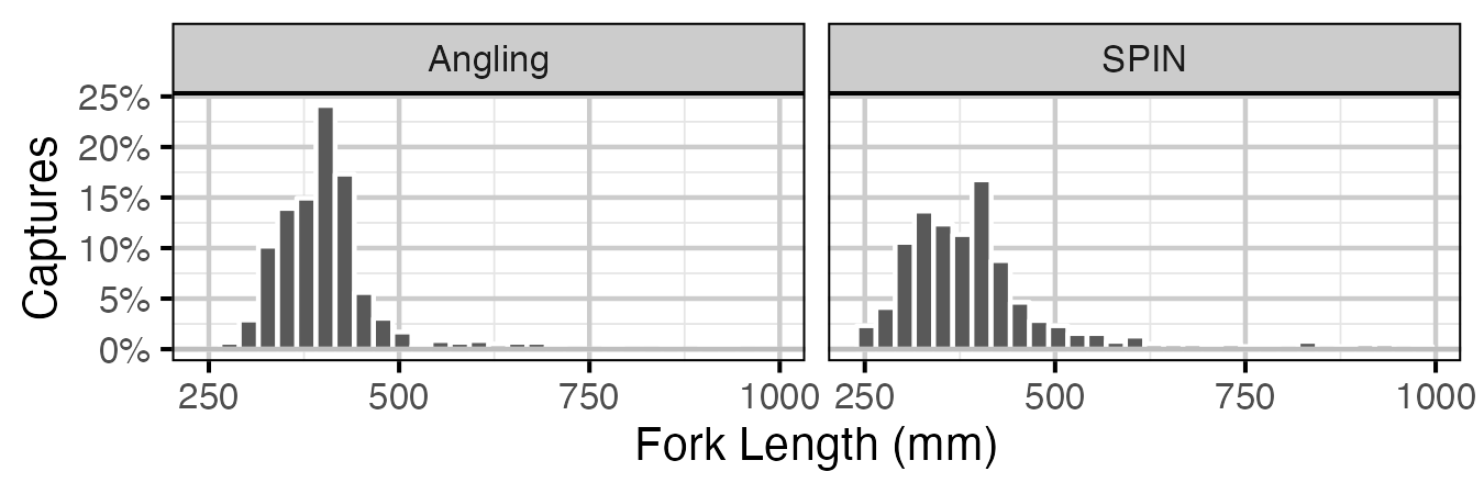
Figure 4. Percentage of fork length (mm) of Lake Trout by method. Only fish greater then 100 mm are shown.
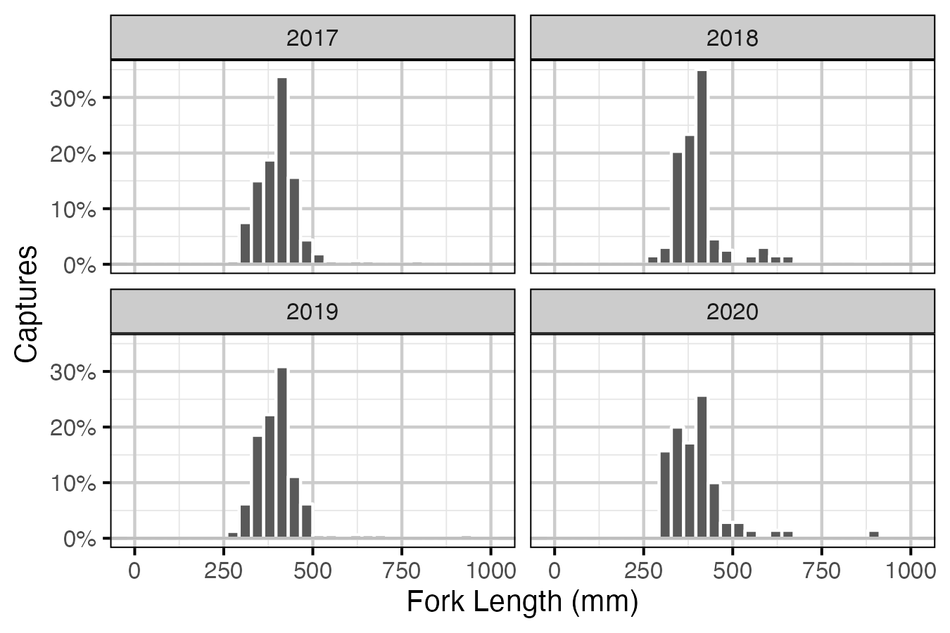
Figure 5. Percentage of fork length (mm) of Lake Trout caught by angling by year. Only fish greater then 100 mm are shown.
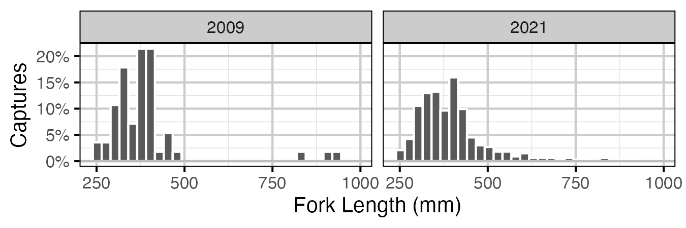
Figure 6. Percentage of fork length (mm) of Lake Trout caught by SPIN survey by year. Only fish greater then 100 mm are shown.
Coverage
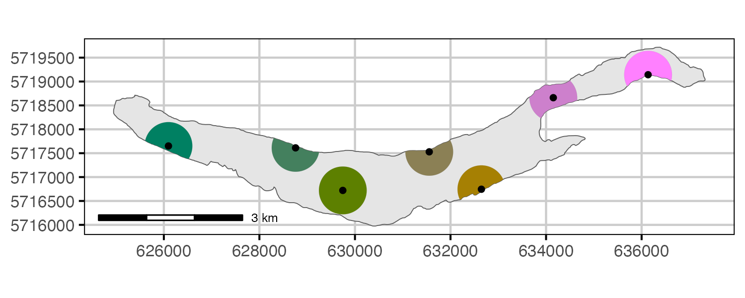
Figure 7. Location of sites with deployed receivers and estimated coverage (500m radius). Although receivers move slightly over time and after being redeployed, the centroid of all known locations for each receiver is shown.
Detections
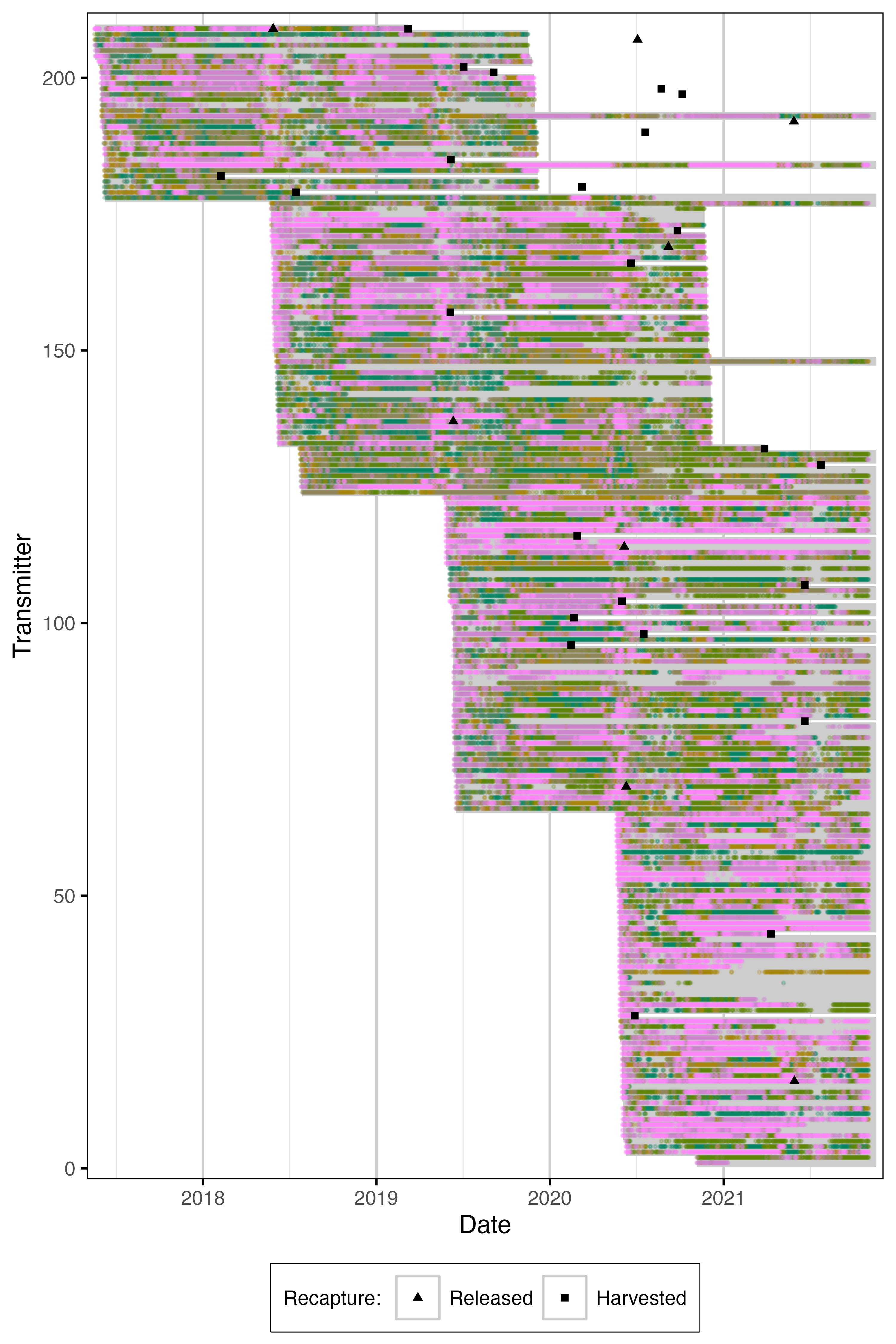
Figure 8. Date of detections by species for each acoustically tagged fish. Grey segments indicate estimated tag life from capture date. Detections have been aggregated daily.
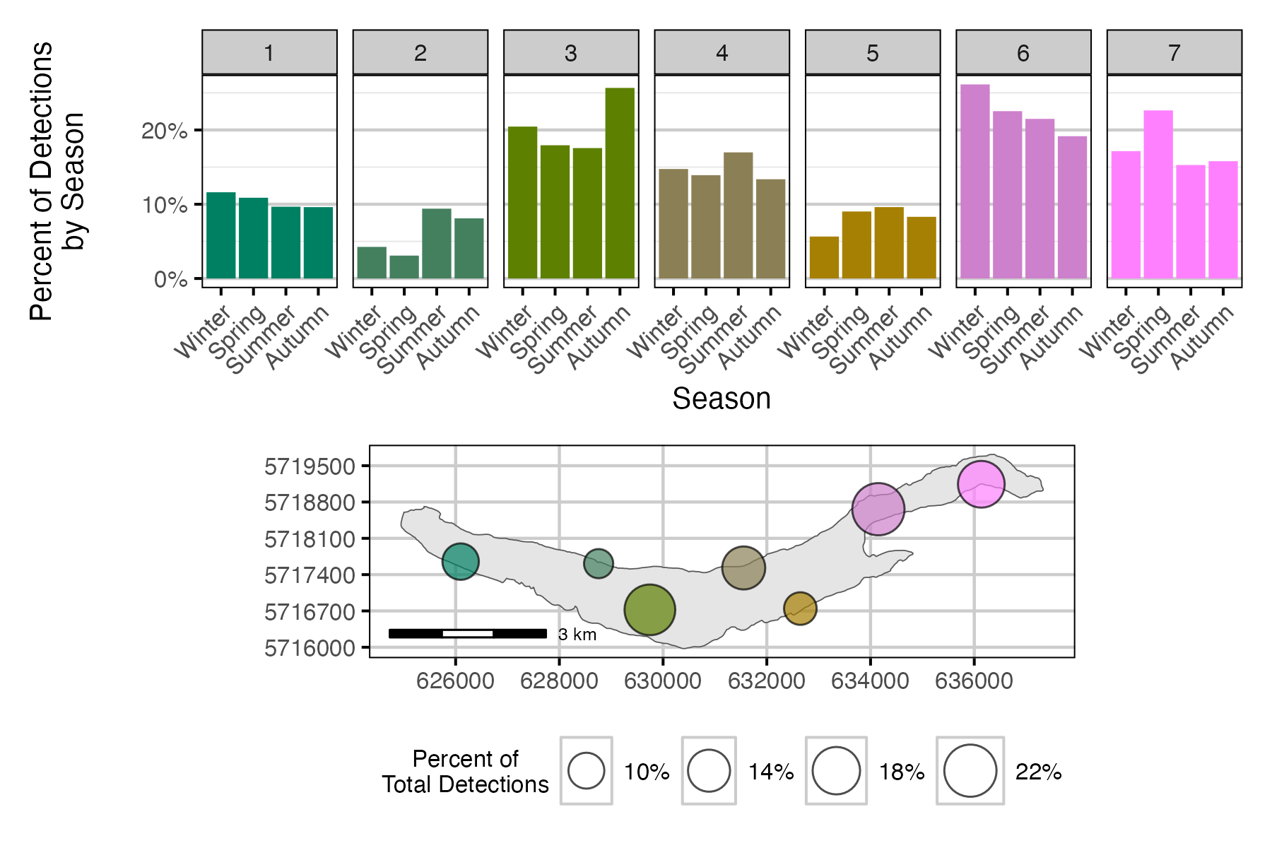
Figure 9. Percent of Lake Trout detections by receiver location and season.
Mobile Detection Survey
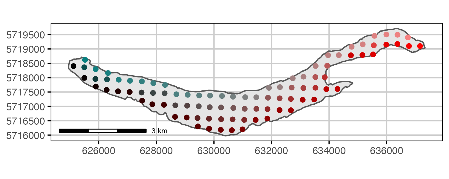
Figure 10. Mobile survey grid locations.
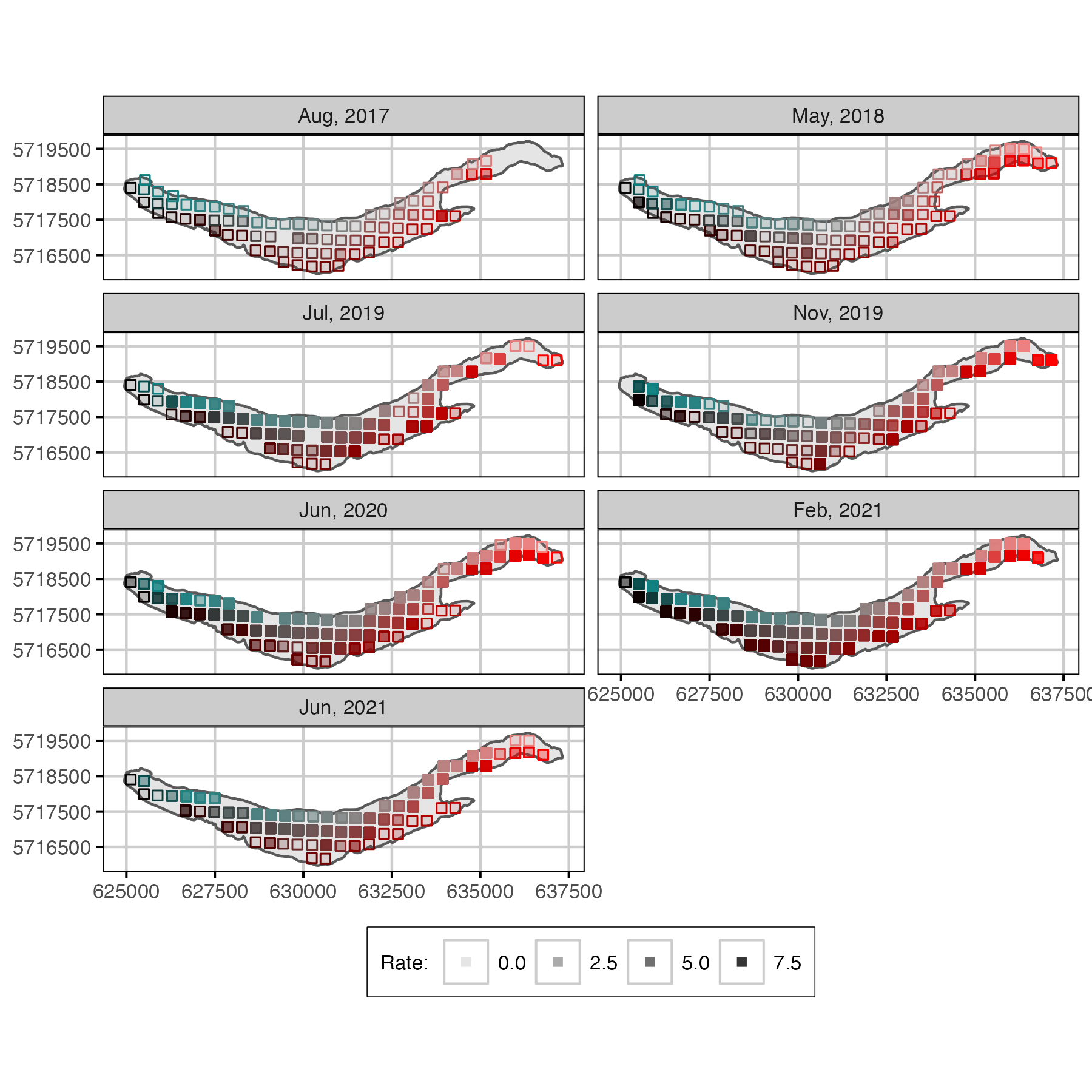
Figure 11. Mobile receiver detection rates (detection/min) for each survey. Missing boxes indicate locations not visit.
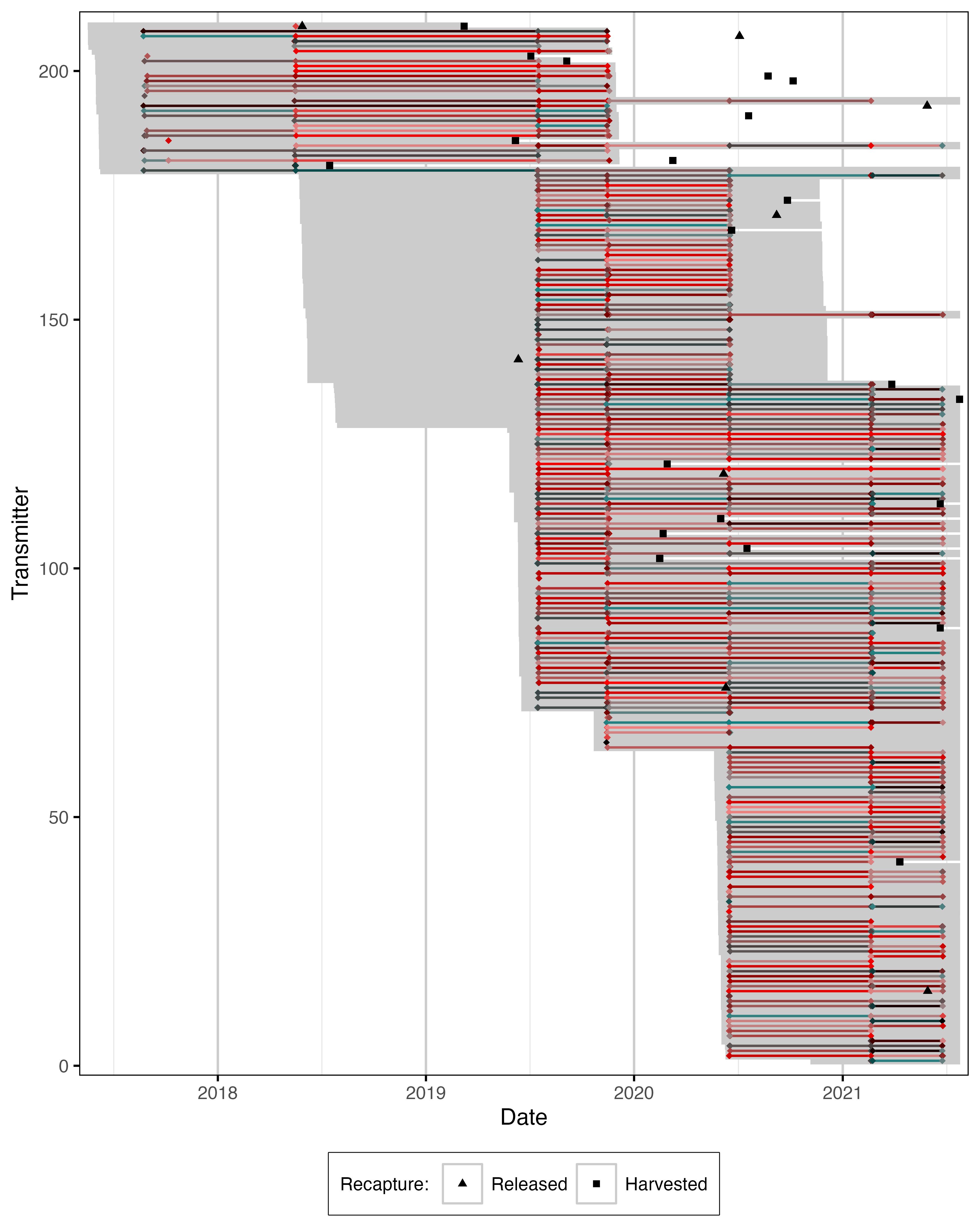
Figure 12. Date of mobile detections for acoustically tagged fish. Grey segments indicate estimated tag life from capture date.
Condition
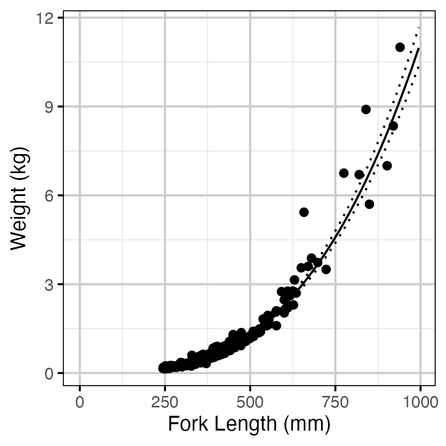
Figure 13. Estimated weight by length (with 95% CIs).
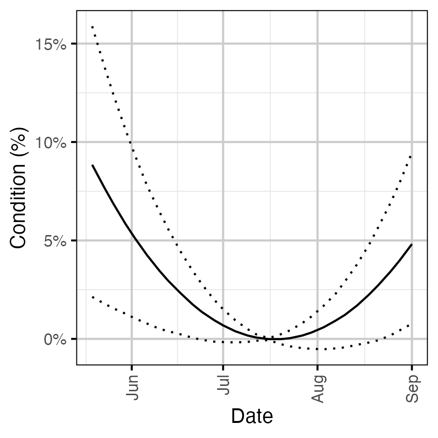
Figure 14. Effect of date on the body condition of a 100 mm fish relative to July 15th (with 95% CIs).
Growth and Spawning
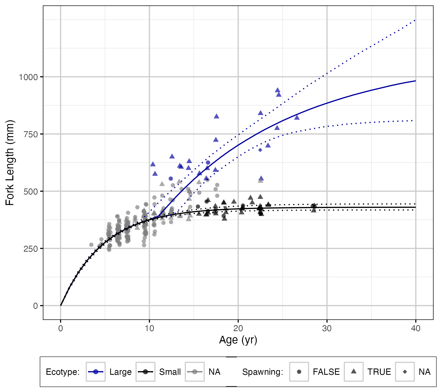
Figure 15. Estimated fork length (mm) by age and ecotype (with 95% CIs).
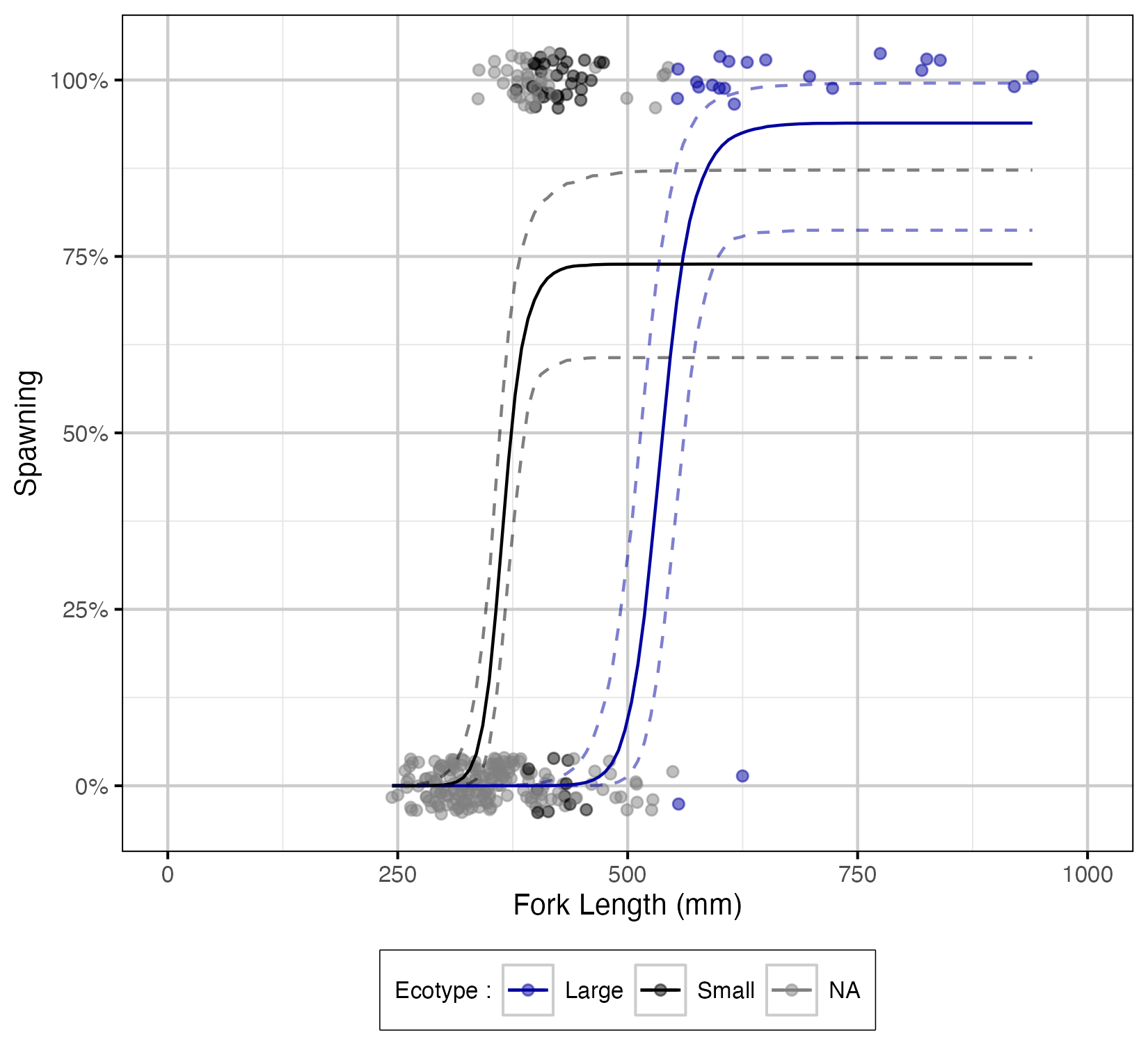
Figure 16. The probability of spawning by fork length (mm) and by Ecotype (with 95% CIs).
Survival
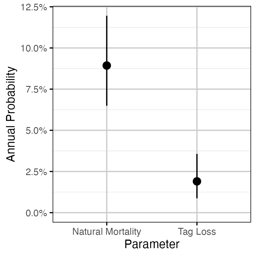
Figure 17. The estimated annual interval probabilities (with 95% CIs).
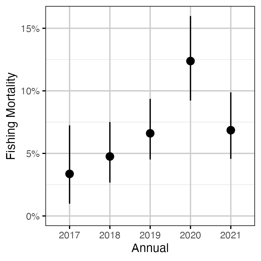
Figure 18. The estimated annual effect on fishing mortality (with 95% CIs).
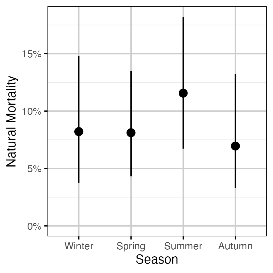
Figure 19. The estimated seasonal effect on natural mortality (with 95% CIs).
Yield-per-Recruit
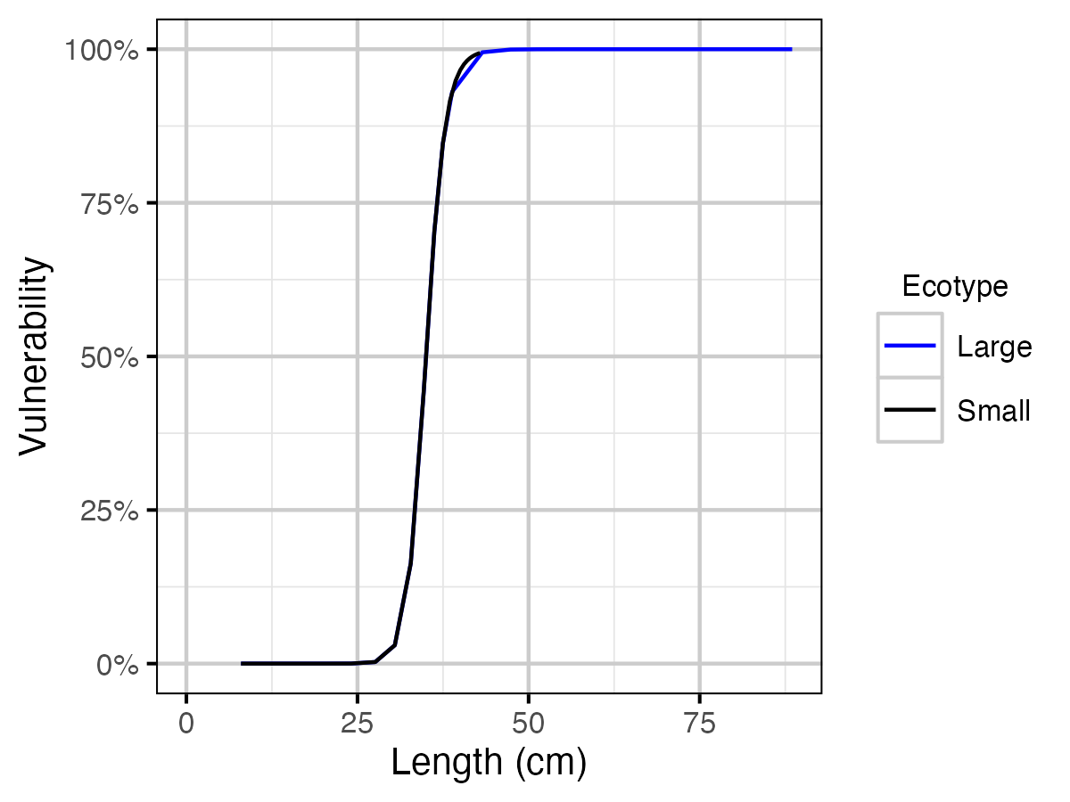
Figure 20. Lake Trout assumed length by vulnerability to capture and ecotype.
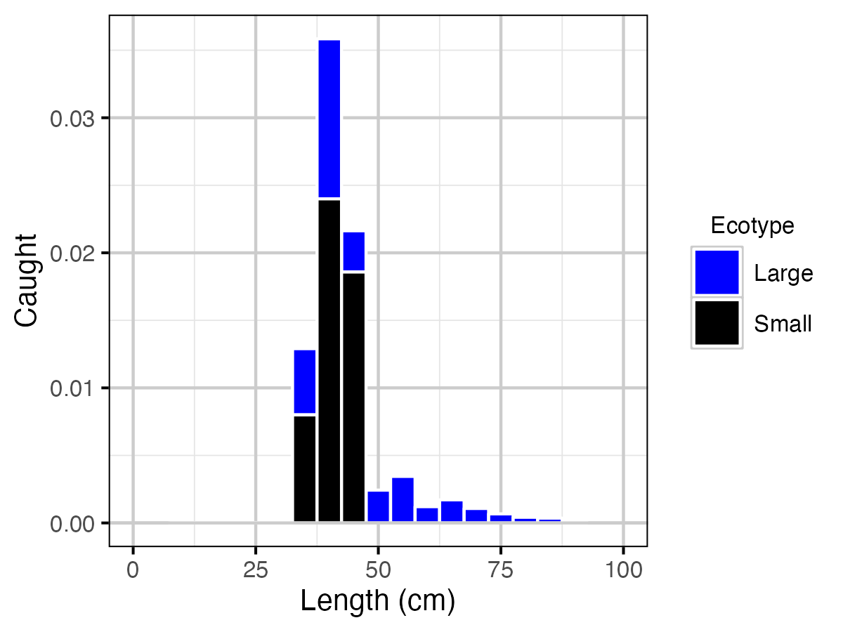
Figure 21. Predicted Lake Trout catch at current estimated explotation rate by length and by ecotype.
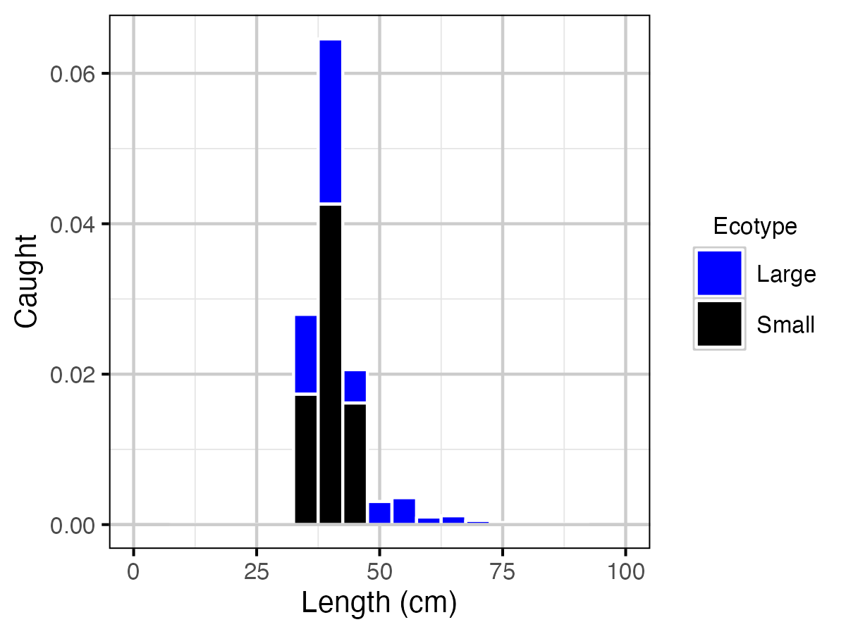
Figure 22. Predicted Lake Trout catch at current estimated optimal explotation rate by length and by ecotype.
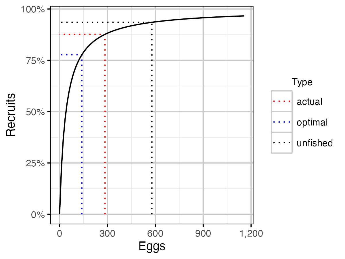
Figure 23. Lake Trout stock recruitment curve.
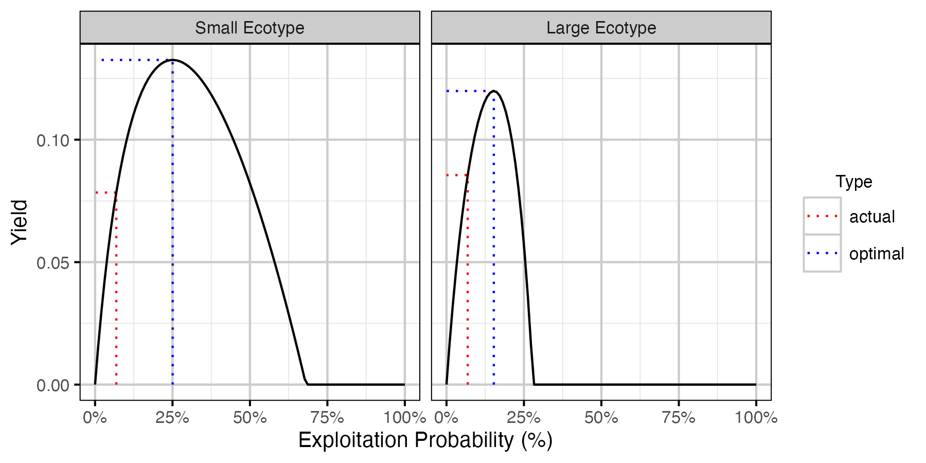
Figure 24. Lake Trout calculated yield as percent of total unfished population by annual interval fishing mortality rate and ecotype.
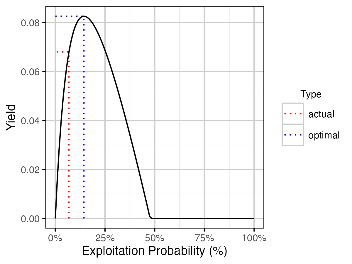
Figure 25. Lake Trout calculated yield as percent of total unfished population by annual interval fishing mortality rate.
Acknowledgements
The organizations and individuals whose contributions have made this analytic appendix possible include:
- Poisson Consulting Ltd.
- Evan Amies-Galonski
- Seb Dalgarno
- MFLNRO - Cariboo Region
- Russ Bobrowski
- Scott Horley