Elk River WCT Abundance Analysis 2022
The suggested citation for this analytic appendix is:
Hill, N.E., Pearson, A.D., & Thorley, J.L. (2023) Elk River WCT Abundance Analysis 2022. A Poisson Consulting Analytic Appendix. URL: https://www.poissonconsulting.ca/f/876409566.
Background
The Elk River is one of eight upper Kootenay River tributaries (Bull, Michel, Skookumchuck, St. Mary, upper Kootenay, White and Wigwam) that are designated as Class II due to the importance of their recreational fisheries for Westslope Cutthroat Trout (Oncorhynchus clarkii lewisi). The population abundance of Westslope Cutthroat Trout in the Elk River is uncertain. To improve population estimates a mark-recapture analysis using Passive Integrated Transponder (PIT) tags deployed by both boat electrofishing and guides was recommended (J. L. Thorley 2021).
After a successful pilot study in 2021, data collection via boat electrofishing and guides continued in 2022. The goal of the present analysis is to use the additional data to get an improved estimate of Westslope Cutthroat Trout population abundance in the Elk River.
Data Preparation
The data were provided by Nupqu Limited Partnership. The data were prepared for analysis using R version 4.2.2 (R Core Team 2022) and organized in a SQLite database. All river distances are based on the BC Freshwater Atlas layer.
Key assumptions of the data preparation included:
- PIT Tag numbers were recorded correctly in instances where the data was not verifiable by the PIT Reader log.
- PIT Reader log was taken to be correct in instances where the recorded PIT Tag code did not match the PIT Reader log.
- 2021 data were submitted in Mountain time; 2022 data were submitted in GMT-6.
- Fork lengths were measured accurately.
- GPS coordinates of outing start/end points were extended if they did not overlaps locations of fish captured on a given outing using the coordinates of a previous outing.
Statistical Analysis
Model parameters were estimated using Bayesian methods. The estimates were produced using JAGS (Plummer 2003) and STAN (Carpenter et al. 2017). For additional information on Bayesian estimation the reader is referred to McElreath (2020).
Unless stated otherwise, the Bayesian analyses used weakly informative normal and half-normal prior distributions (Gelman, Simpson, and Betancourt 2017). The posterior distributions were estimated from 1500 Markov Chain Monte Carlo (MCMC) samples thinned from the second halves of 3 chains (Kery and Schaub 2011, 38–40). Model convergence was confirmed by ensuring that the potential scale reduction factor \(\hat{R} \leq 1.05\) (Kery and Schaub 2011, 40) and the effective sample size (Brooks et al. 2011) \(\textrm{ESS} \geq 150\) for each of the monitored parameters (Kery and Schaub 2011, 61).
Model adequacy was assessed via posterior predictive checks (Kery and Schaub 2011). More specifically, the proportion of zeros in the data and the first four central moments (mean, variance, skewness and kurtosis) in the deviance residuals were compared to the expected values by simulating new data based on the posterior distribution and assumed sampling distribution and calculating the deviance residuals.
Where computationally practical, the sensitivity of the posteriors to the choice of prior distributions was evaluated by increasing the standard deviations of all normal, half-normal and log-normal priors by an order of magnitude and then using \(\hat{R}\) to evaluate whether the samples were drawn from the same posterior distribution (Joseph L. Thorley and Andrusak 2017).
The parameters are summarised in terms of the point estimate, lower and upper 95% compatibility limits (Rafi and Greenland 2020) and the surprisal s-value (Greenland 2019). The estimate is the median (50th percentile) of the MCMC samples while the 95% CLs are the 2.5th and 97.5th percentiles. The s-value indicates how surprising it would be to discover that the true value of the parameter is in the opposite direction to the estimate (Greenland 2019). An s-value of \(>\) 4.32 bits, which is equivalent to a p-value \(<\) 0.05 (Kery and Schaub 2011; Greenland and Poole 2013), indicates that the surprise would be equivalent to throwing at least 4.3 heads in a row.
Model selection was based the heuristic of directional certainty (Kery and Schaub 2011). Fixed effects were included if their s-value was \(>\) 4.32 bits (Kery and Schaub 2011). Based on a similar argument, random effects were included if their standard deviation had lower 95% CLs \(>\) 5% of the estimate.
The results are displayed graphically by plotting the modeled relationships between individual variables and the response with the remaining variables held constant. In general, continuous and discrete fixed variables are held constant at their mean and first level values, respectively, while random variables are held constant at their average values (expected values of the underlying hyperdistributions) (Kery and Schaub 2011, 77–82). Primary explanatory variables are evaluated based on their estimated effect sizes with 95% CLs (Bradford, Korman, and Higgins 2005)
The analyses were implemented using R version 4.2.2
(R Core Team 2022) and the
mbr family of packages.
Model Descriptions
Mark-Recapture
The data were analysed using a hierarchical Bayesian mark-recapture abundance model. Each zone was split into two kilometres sites except sites at the end of the zone were added to the previous site if the length was less than one kilometre. Captures from sites that had less then 10% of their length surveyed were not included in the analysis.
Key assumptions of the mark-recapture model include:
- Lineal density varies randomly by year and zone within year.
- There is no movement of marked fish between sites within a sampling season.
- There is no mortality of fish within a sampling season.
- The probability of capturing a marked or unmarked fish is the same.
- All recaptured fish are correctly identified as being marked and there is no tag loss.
- Capture efficiency varies by electrofishing effort.
- Capture efficiency varies randomly by site visit.
- The number of recaptures (of fish marked at that site in that year) and the total number of fish caught are each binomially distributed.
Model Templates
Mark-Recapture
.model{
  bDensity ~ dnorm(6, 2^-2)
  bEfficiency ~ dnorm(-5, 2^-2)
  bEfficiencySecondsPerMetre ~ dnorm(0, 1^-2)
  bTheta ~ dexp(10)
  bDensityAnnual[1] <- 0
  for (i in 2:nannual) {
    bDensityAnnual[i] ~ dnorm(0, 2^-2)
  }
  sDensityAnnualZoneID ~ dnorm(0, 1^-2) T(0,)
  for (i in 1:nannual) {
    for (j in 1:nzone_id) {
      bDensityAnnualZoneID[i, j] ~ dnorm(0, sDensityAnnualZoneID^-2)
    }
  }
  bEfficiencyAnnual[1] <- 0
  for (i in 2:nannual) {
    bEfficiencyAnnual[i] ~ dnorm(0, 2^-2)
  }
  for (i in 1:nObs) {
    log(eDensity[i]) <- bDensity + bDensityAnnual[annual[i]] + bDensityAnnualZoneID[annual[i], zone_id[i]]
    logit(eProb[i]) <- bEfficiency + bEfficiencySecondsPerMetre * seconds_per_metre[i] + bEfficiencyAnnual[annual[i]]
    eEfficiency[i] ~ dbeta((2 * eProb[i]) / bTheta, (2 * (1 - eProb[i])) / bTheta)
    recaptures[i] ~ dbin(eEfficiency[i], marked[i])
    bAbundance[i] ~ dpois(eDensity[i] * site_length[i] * survey_proportion[i])
    count[i] ~ dbin(eEfficiency[i], bAbundance[i])
  }
Block 1. Model description.
Results
Tables
Mark-Recapture
Table 1. Parameter descriptions.
| Parameter | Description |
|---|---|
annual[i] |
Year of the ith survey visit |
bAbundance[i] |
Expected abundance during ith site visit |
bDensityAnnualZoneID[i, j] |
Effect of the ith year and the jth zone on
bDensity |
bDensityAnnual[i] |
Effect of ith year on bDensity |
bDensity |
Intercept of log(eDensity) |
bEfficiencyAnnual[i] |
Effect of ith year on logit(eProb) |
bEfficiencySecondsPerMetre |
Effect of electrofishing seconds per metre
travelled on eEfficiency |
bEfficiency |
Intercept for logit(eEfficiency) |
bTheta |
Variation in the random effect of site visit on
eEfficiency |
count[i] |
The number of fish captured during the ith
site visit |
eDensity[i] |
Expected fish density during the ith site
visit |
eEfficiency[i] |
Expected capture efficiency including the random effect of site visit |
eProb[i] |
Expected capture efficiency during the ith
site visit |
marked[i] |
Number of fish marked prior to the ith site
visit |
recaptures[i] |
Number of marked fish observed during the ith
site visit |
seconds_per_metre[i] |
Number of electrofishing seconds per metre on the
ith site visit |
site_length[i] |
Length of the site visited for the ith site
visit |
survey_proportion[i] |
Proportion of site surveyed during the ith
site visit |
zone_id[i] |
Zone of the ith survey visit |
Table 2. Model coefficients.
| term | estimate | lower | upper | svalue |
|---|---|---|---|---|
| bDensity | 5.88000 | 5.0300 | 6.7000 | 10.6000 |
| bDensityAnnual[2] | -0.00432 | -0.8500 | 1.0900 | 0.0174 |
| bEfficiency | -5.44000 | -6.0100 | -4.8700 | 10.6000 |
| bEfficiencyAnnual[2] | 1.03000 | 0.5010 | 1.5600 | 10.6000 |
| bEfficiencySecondsPerMetre | 0.20400 | 0.0507 | 0.3540 | 6.4600 |
| bTheta | 0.01910 | 0.0122 | 0.0292 | 10.6000 |
| sDensityAnnualZoneID | 0.40000 | 0.1020 | 0.9990 | 10.6000 |
Table 3. Model convergence.
| n | K | nchains | niters | nthin | ess | rhat | converged |
|---|---|---|---|---|---|---|---|
| 188 | 7 | 3 | 500 | 5000 | 156 | 1.01 | TRUE |
Table 4. The estimated abundance of WCT in zones 2 to 6 on Elk River, by year (with 95% CIs).
| annual | estimate | lower | upper |
|---|---|---|---|
| 2021 | 35125.60 | 19755.97 | 67838.93 |
| 2022 | 32167.51 | 23676.28 | 46452.53 |
Table 5. Model posterior predictive checks.
| moment | observed | median | lower | upper | svalue |
|---|---|---|---|---|---|
| zeros | 0.3031915 | 0.2340426 | 0.1595745 | 0.3138298 | 3.8934968 |
| mean | -1.0171159 | -0.9137361 | -1.0081736 | -0.8258678 | 4.9971194 |
| variance | 0.3130478 | 0.3714921 | 0.2921255 | 0.4683314 | 2.6999592 |
| skewness | -0.6425487 | -0.6136020 | -1.0146960 | -0.3480178 | 0.2152017 |
| kurtosis | 0.2399603 | -0.0390868 | -0.6950496 | 1.7591280 | 0.7109303 |
Table 6. Model sensitivity.
| all | analysis | sensitivity | bound |
|---|---|---|---|
| all | 1.01 | 1.027 | 1.018 |
Figures
Maps
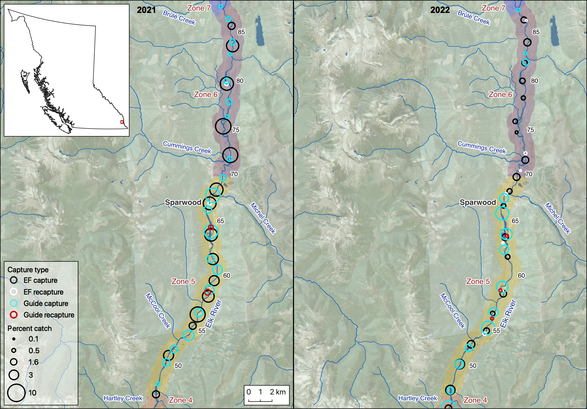
Figure 1. A map showing the percentage of captures on Elk River, by capture method and year. The percentage of electrofishing captures at a given site was weighted by the number of site visits.
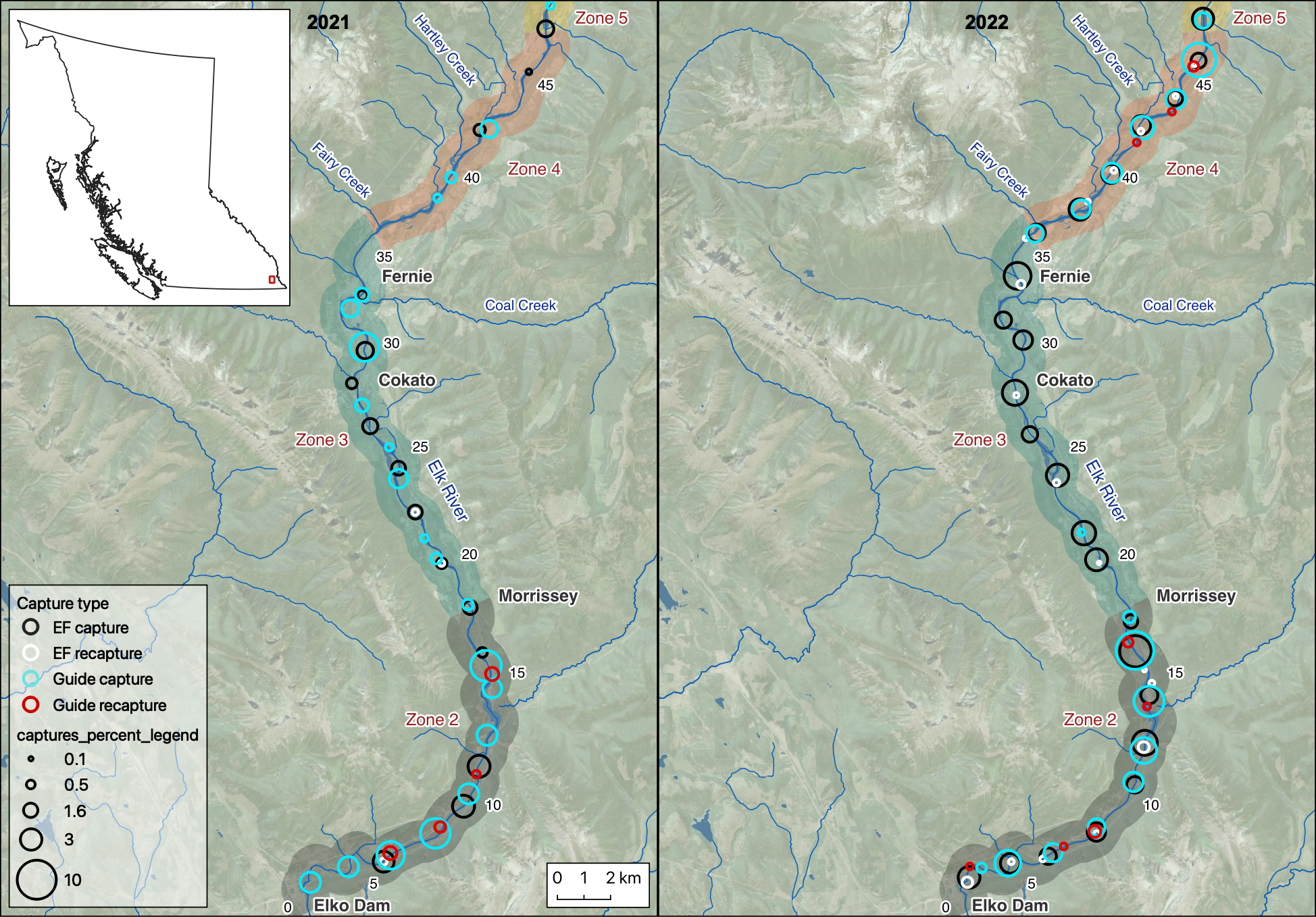
Figure 2. A map showing the percentage of captures on Elk River, by capture method and year. The percentage of electrofishing captures at a given site was weighted by the number of site visits.
Size
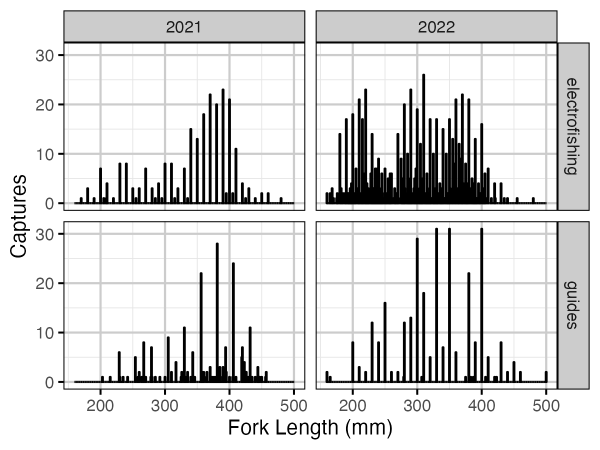
Figure 3. Fork lengths (in mm) of fish caught by electrofishing and guides by year.
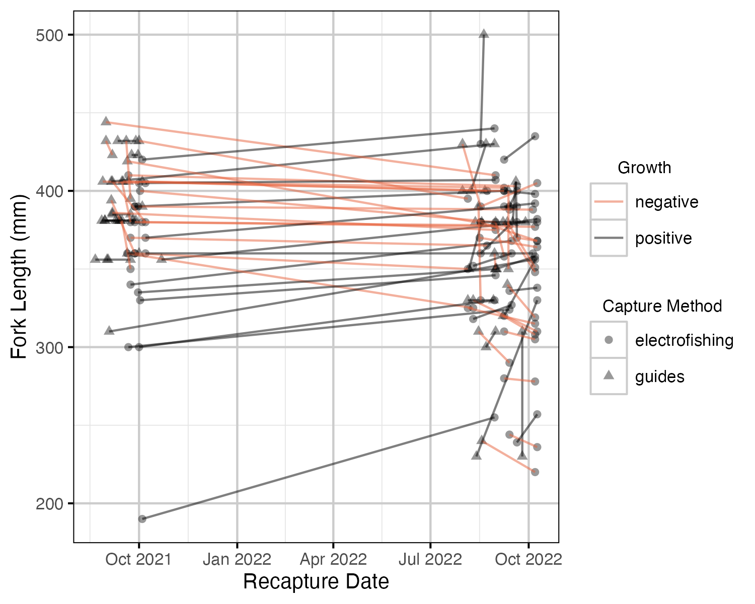
Figure 4. Fork lengths of recaptured fish over time.
Captures
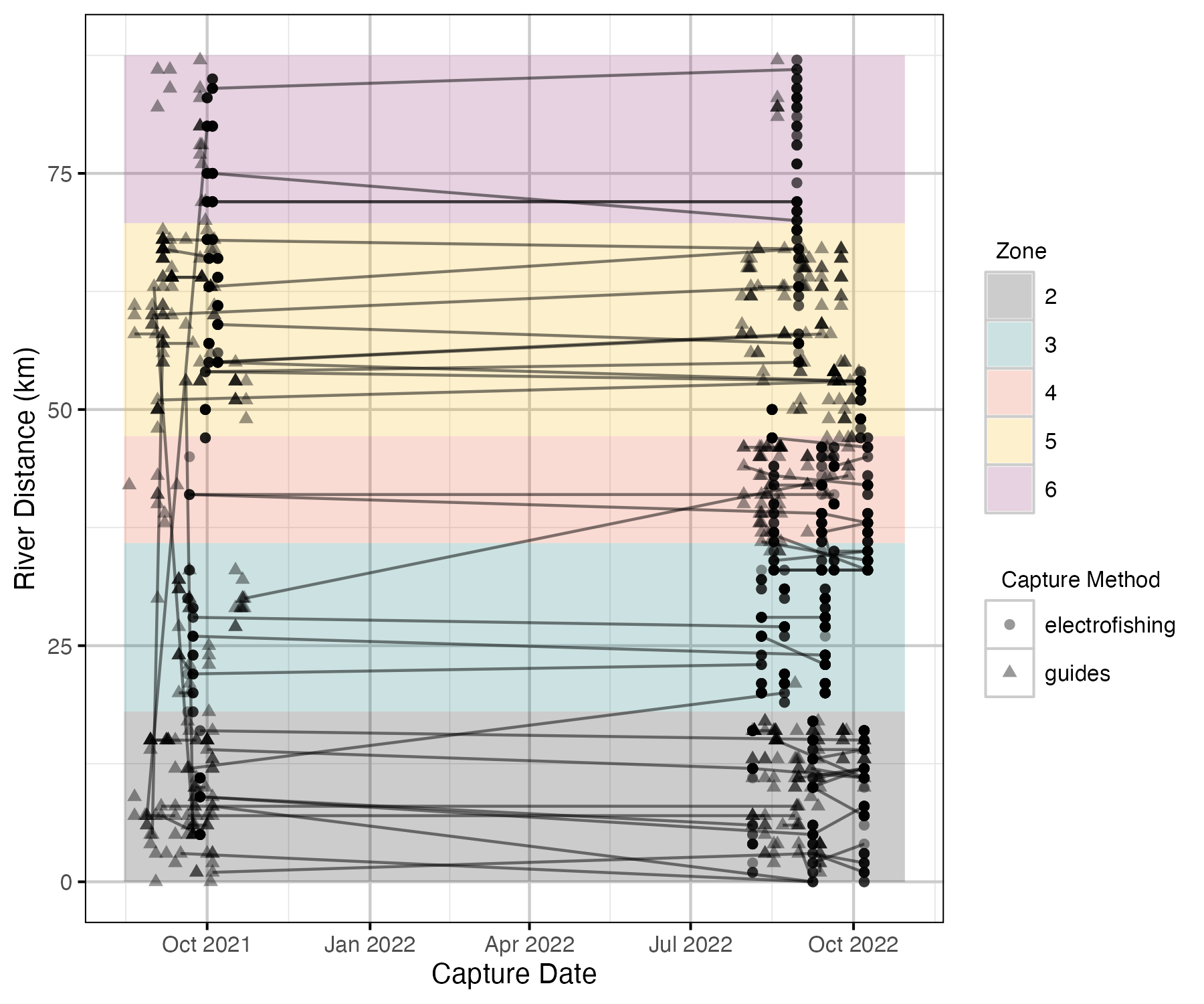
Figure 5. Locations of captures and recaptures along Elk River over time.
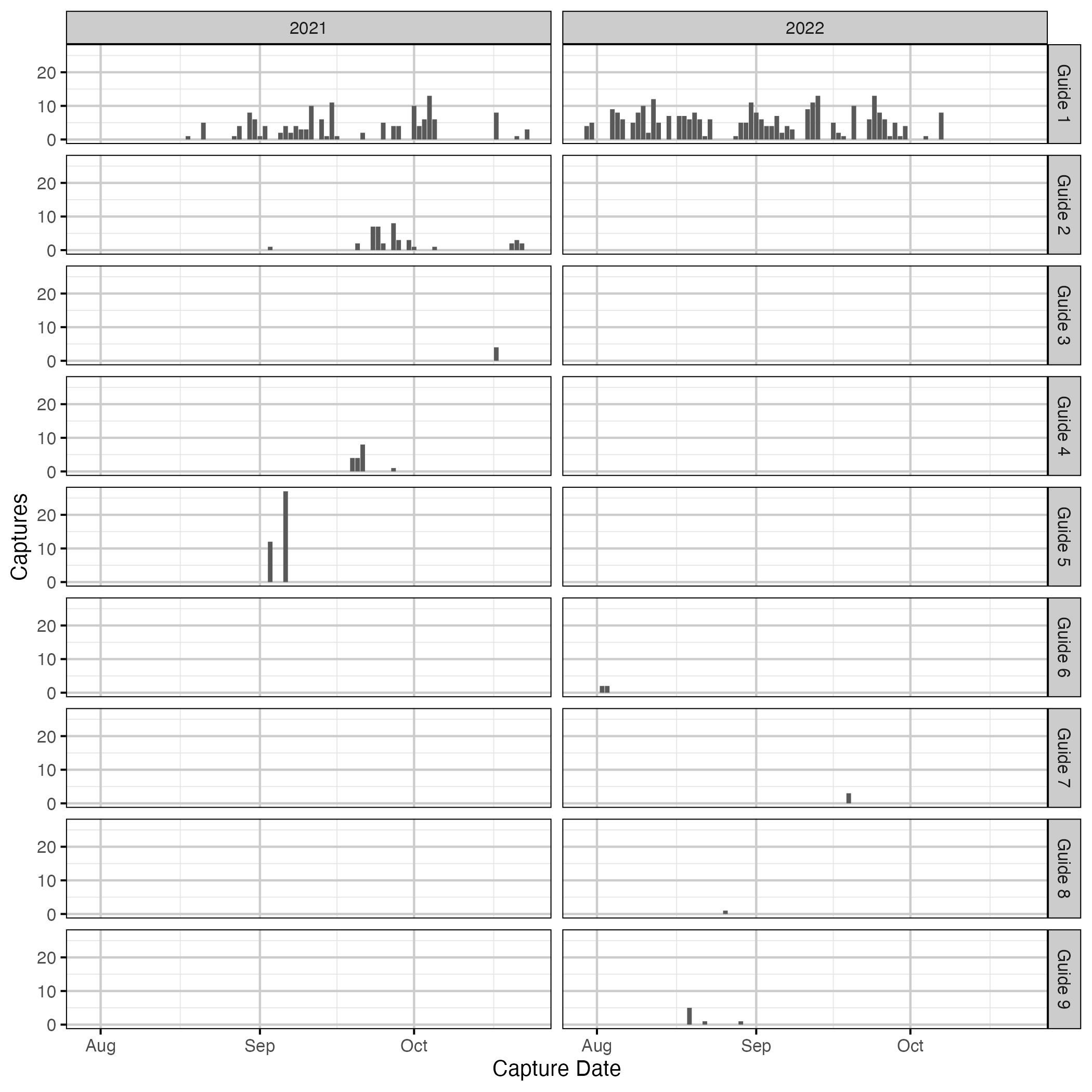
Figure 6. Number of captures by guides over time.
Mark-Recapture
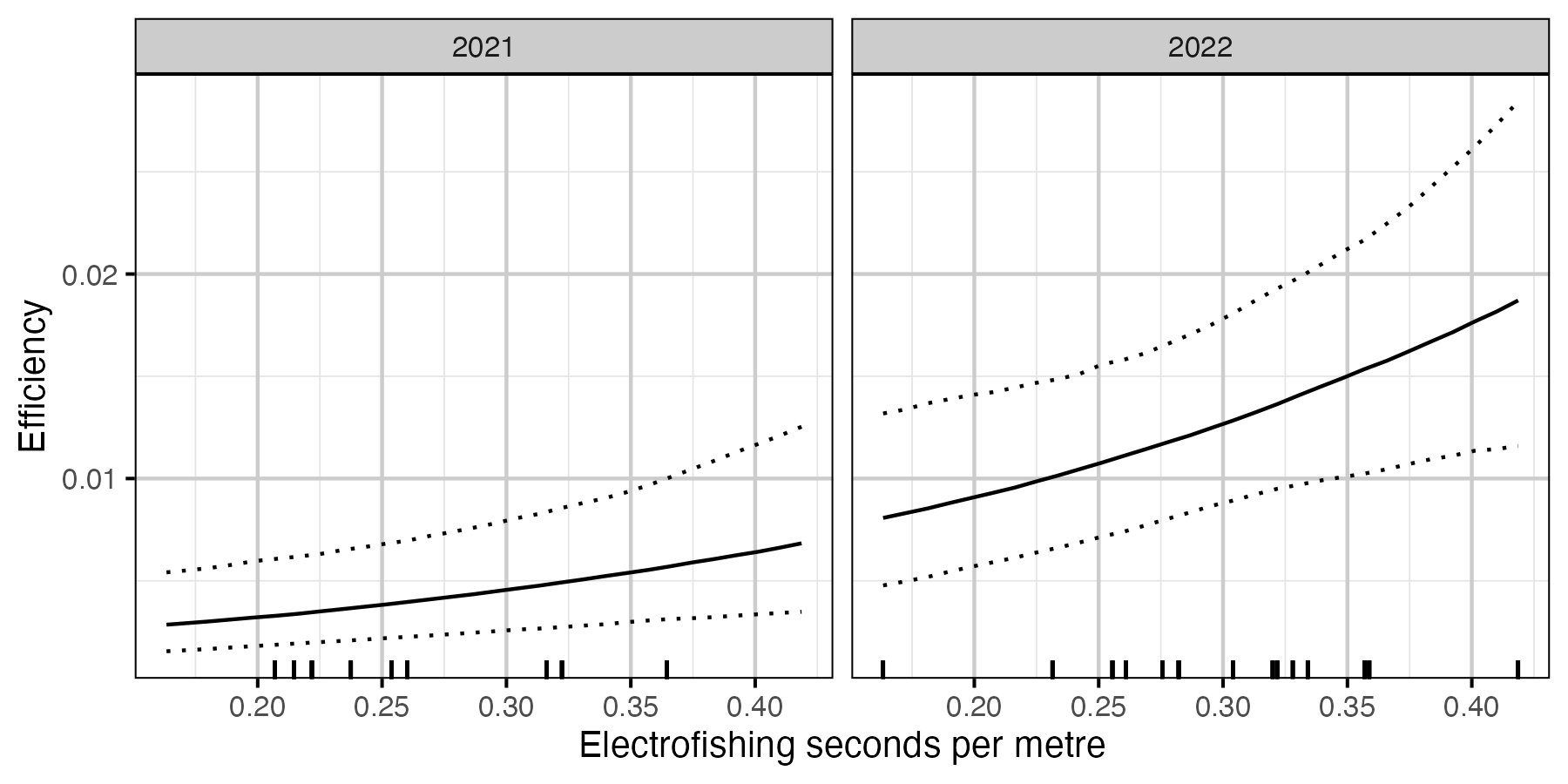
Figure 7. The estimated relationship between seconds of electrofishing and capture efficiency (with 95% CIs). The dashes along the x-axis represent the data.
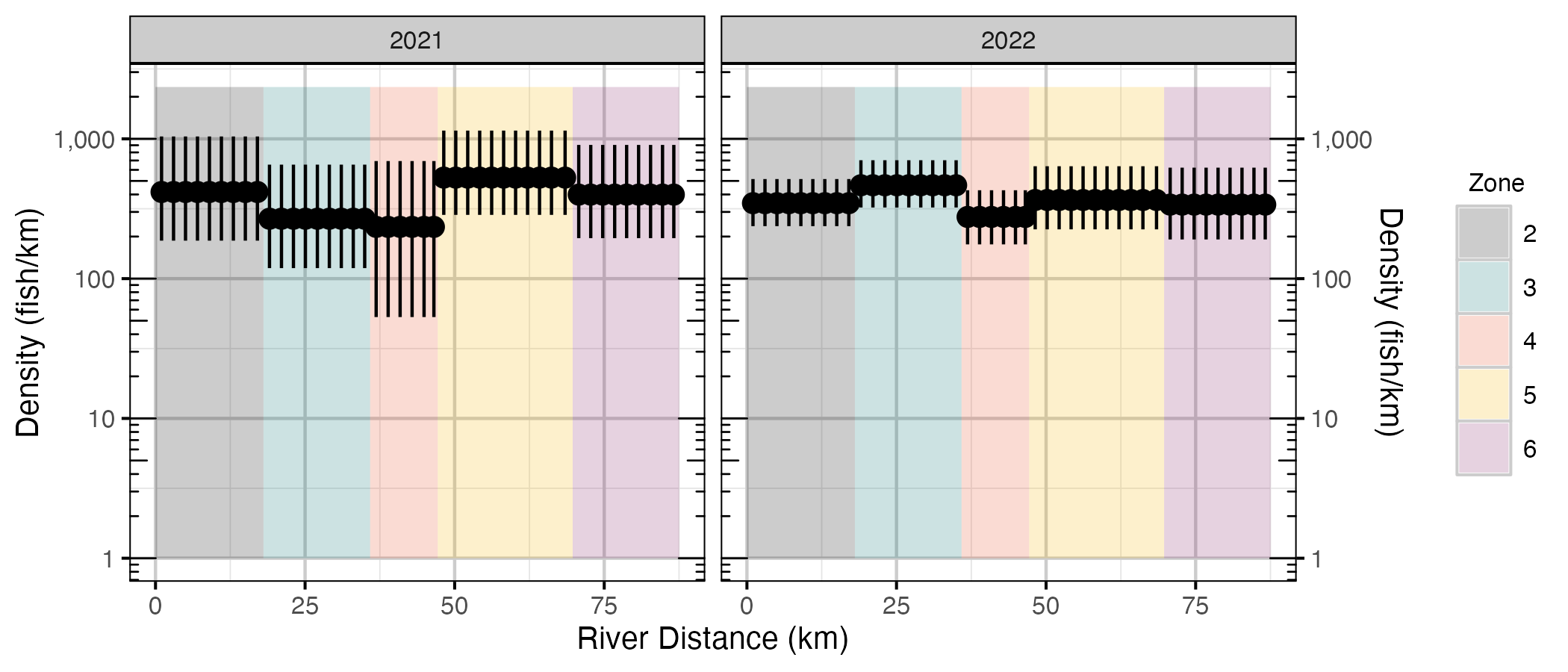
Figure 8. The estimated lineal density (on a log scale) of WCT on Elk River by river distance, zone, and year (with 95% CIs).
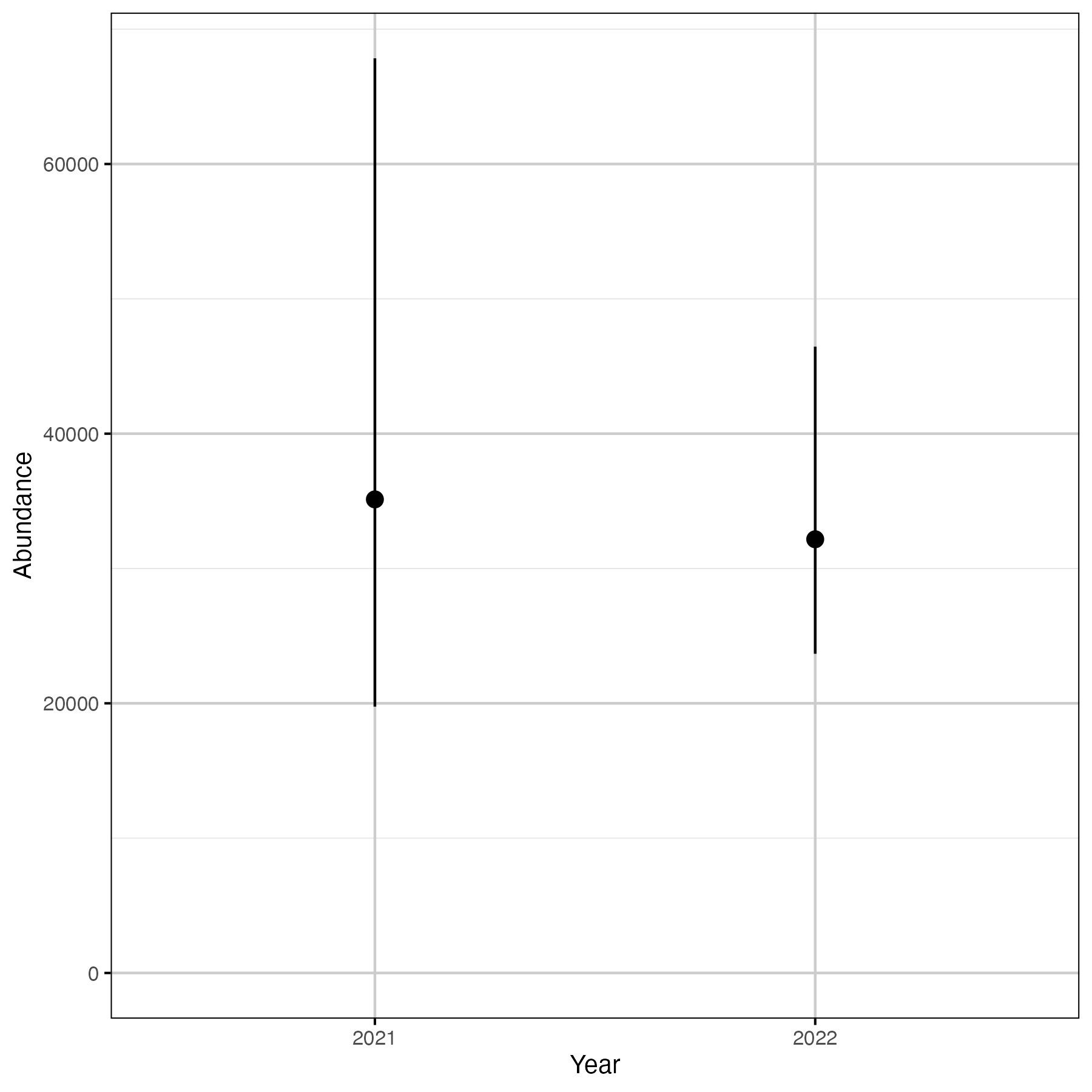
Figure 9. The estimated abundance of WCT in the Elk River, by year (with 95% CIs).
Outing
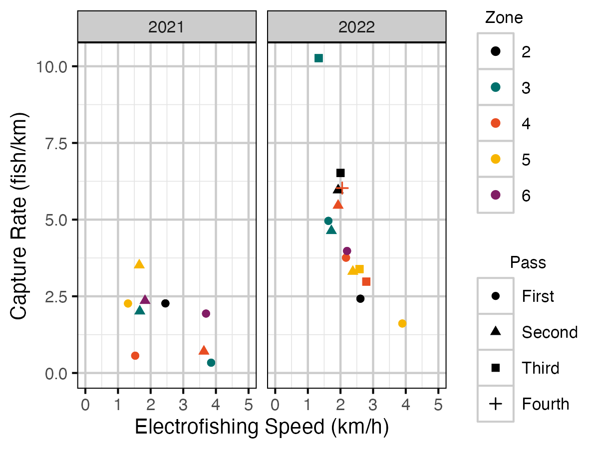
Figure 10. Rate fish were caught per kilometre by the speed (km/h) electrofishing crews floated down Elk River for each outing.
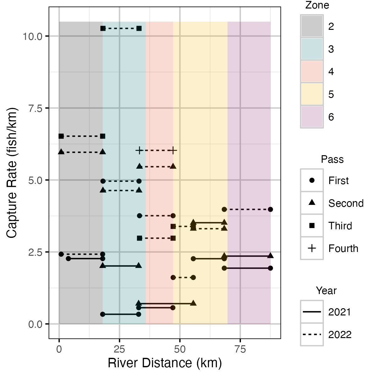
Figure 11. The rate electrofishing crews caught fish per kilometre by river distance (km) for each outing.
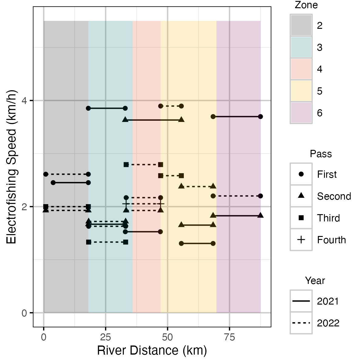
Figure 12. Rate of kilometres per hour electrofishing crews floated down Elk River for each outing.
Codes
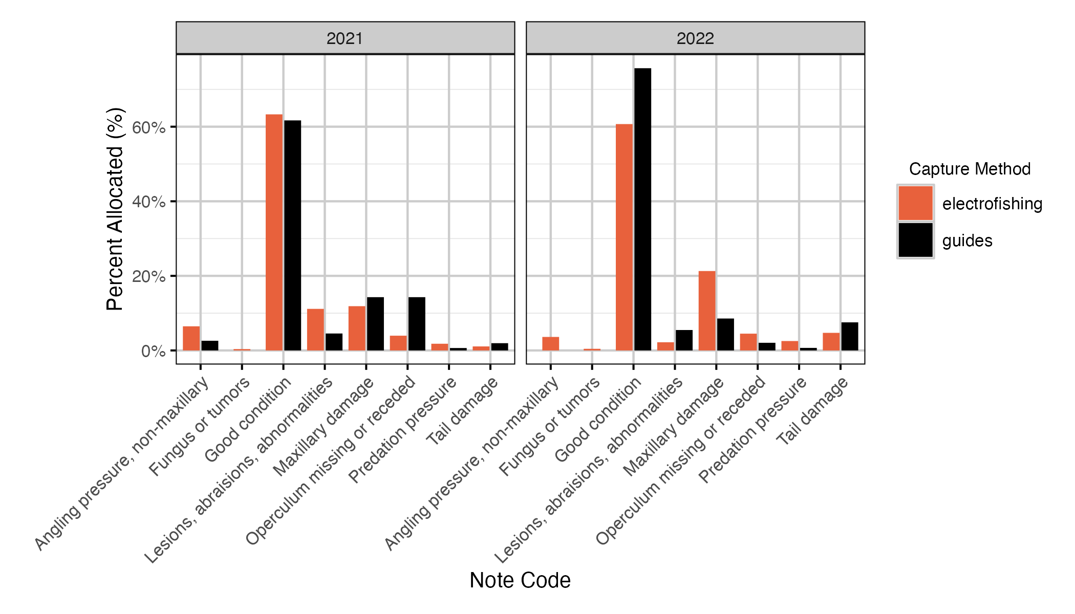
Figure 13. The percentage of note codes allocated to fish by capture method and year. The fish in the ‘guides’ group are those caught by Guide 1 only.
Recommendations
Recommendations include:
- Measure and record fork length to 1 mm.
- Use a unique naming convention for photo file names, as a
combination of the capture date-time, reader ID, PIT Tag code and
photo type (R = reader; F = fish left; D = damage)
- YYYY-MM-DD-hhmmss_readerID_PITTagCode_PhotoType
- e.g., 2020-07-23-131042_6_900088000907916_R
- Develop a growth model that incorporates measurement error.
Acknowledgements
The organizations and individuals whose contributions have made this analytic appendix possible include:
- Nupqu Limited Partnership
- Mark Fjeld
- Dominique Nicholas
- Rafael Lugo
- Teck Coal Ltd.
- Bronwen Lewis
- Dorian Turner
- BC Government
- Matt Neufeld
- Will Warnock