Duncan Lardeau Juvenile Rainbow Trout Abundance 2017
The suggested citation for this analytic report is:
Thorley, J.L., Andrusak, G.F., Muir, C.D., Dalgarno, S. and Hogan P.M. (2017) Duncan Lardeau Juvenile Rainbow Trout Abundance 2017. A Poisson Consulting Analysis Report. URL: https://www.poissonconsulting.ca/f/492093238.
Background
Rainbow Trout rear in the Lardeau and Lower Duncan rivers. Since 2006 (with the exception of 2015) annual spring snorkel surveys have been conducted to estimate the abundance and distribution of age-1 Rainbow Trout. From 2006 to 2010 the surveys were conducted at fixed index site. Since 2011 fish observations have been mapped to the river based on their spatial coordinates as recorded by GPS.
The primary aims of the current analyses are to:
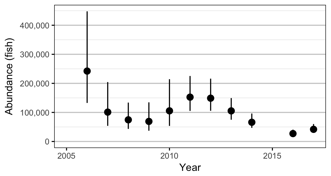
- Estimate the spring abundance of age-1 fish by year.
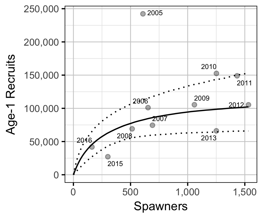
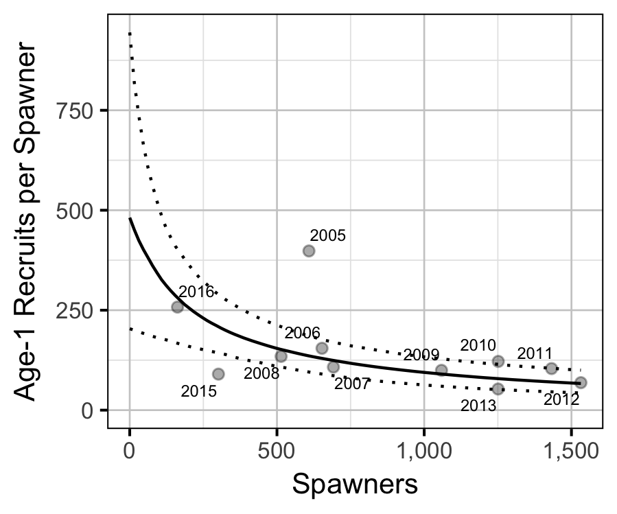
- Estimate the stock-recruitment relationship between the number of spawners and the abundance of age-1 recruits the following spring.
Methods
Data Preparation
The data were provided by the Ministry of Forests, Lands and Natural Resource Operations (MFLNRO). The historical and current snorkel count data were manipulate using R version 3.4.2 (R Core Team 2017) and organised in an SQLite database. Due to the loss of the primary data manager, the estimates should be considered preliminary until additional verification of the restructured data has been conducted. Age-1 individuals were assumed to be those with a fork length \(\geq\) 100 mm.
Data Analysis
Hierarchical Bayesian models were fitted to the data using R version
3.4.2 (R Core Team 2017), Stan 2.16.0 (Carpenter et al. 2017) and
JAGS 4.2.0 (Plummer 2015) and the
mbr family of packages.
Unless indicated otherwise, the models used prior distributions that were vague in the sense that they did not affect the posterior distributions (Kery and Schaub 2011, 36). The posterior distributions were estimated from 2,000 Markov Chain Monte Carlo (MCMC) samples thinned from the second halves of three chains (Kery and Schaub 2011, 38–40). Model convergence was confirmed by ensuring that \(\hat{R} < 1.1\) (Kery and Schaub 2011, 40) for each of the monitored parameters in the model (Kery and Schaub 2011, 61). Where relevant, model adequacy was confirmed by examination of residual plots.
The posterior distributions of the fixed (Kery and Schaub 2011, 75) parameters are summarised in terms of the point estimate, standard deviation (sd), the z-score, lower and upper 95% confidence/credible limits (CLs) and the p-value (Kery and Schaub 2011, 37, 42). The estimate is the median (50th percentile) of the MCMC samples, the z-score is \(\mathrm{mean}/\mathrm{sd}\) and the 95% CLs are the 2.5th and 97.5th percentiles. A p-value of 0.05 indicates that the lower or upper 95% CL is 0.
Variable selection was achieved by dropping fixed (Kery and Schaub 2011, 77–82) variables with two-sided p-values \(\geq\) 0.05 (Kery and Schaub 2011, 37, 42) and random variables with percent relative errors \(\geq\) 80%.
The results are displayed graphically by plotting the modeled relationships between particular variables and the response with 95% credible intervals (CIs) with the remaining variables held constant. In general, continuous and discrete fixed variables are held constant at their mean and first level values respectively while random variables are held constant at their typical values (expected values of the underlying hyperdistributions) (Kery and Schaub 2011, 77–82). Where informative the influence of particular variables is expressed in terms of the effect size (i.e., percent change in the response variable) with 95% CIs (Bradford et al. 2005).
Model Descriptions
Abundance
The abundance was estimated from the count data using an overdispersed Poisson model (Kery and Schaub 2011, 55–56). The annual abundance estimates represent the total number of fish in the study area.
Key assumptions of the abundance model include:
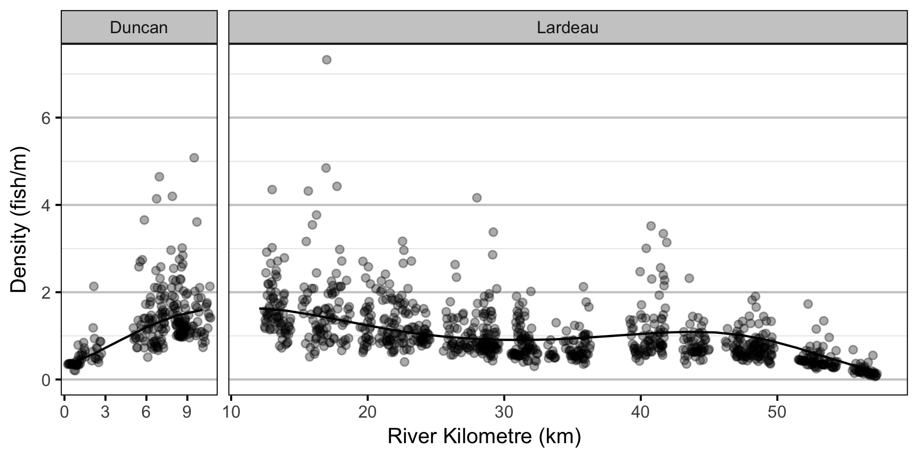
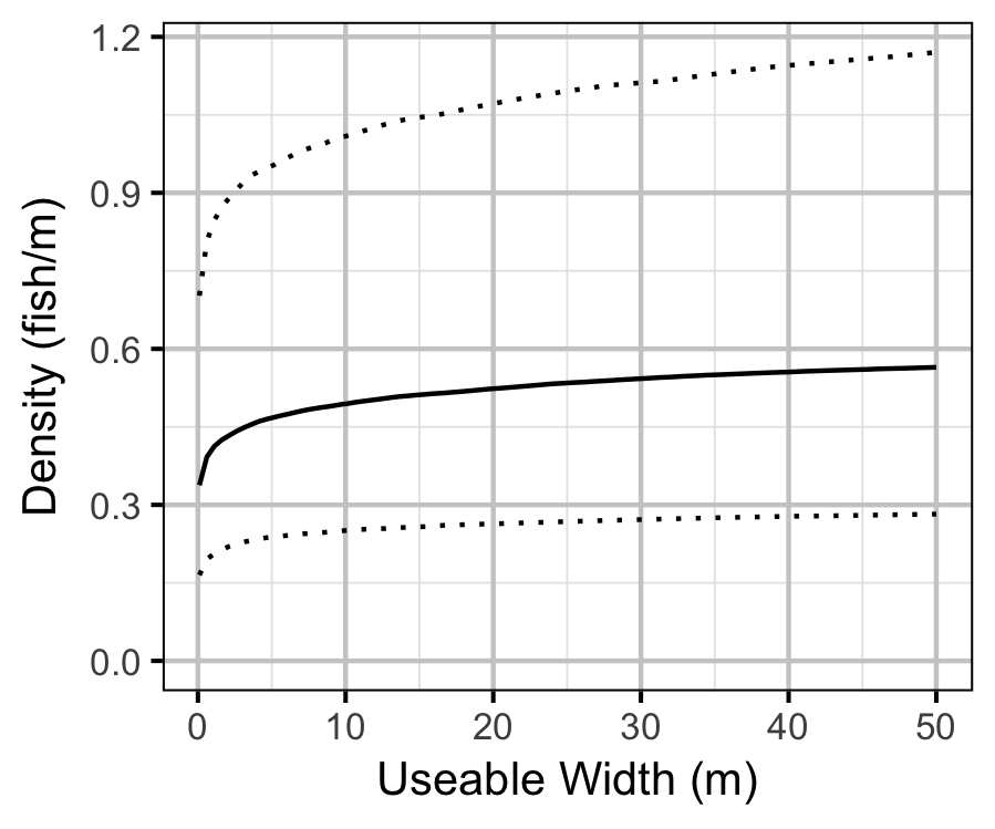
- The lineal fish density varies with year, useable width and river kilometer as a polynomial, and randomly with site.
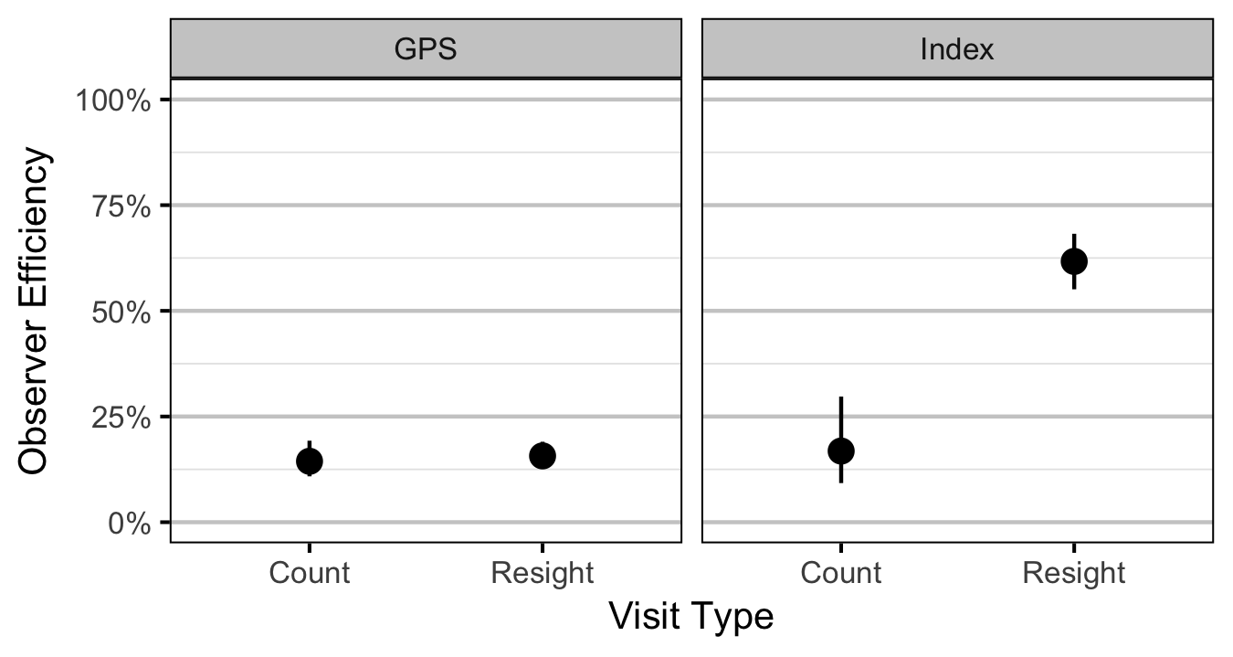
- The observer efficiency at marking sites varies by study design (GPS versus Index).
- The observer efficiency also varies by visit type (marking versus count) within study design and randomly by snorkeller.
- The expected count at a site is the expected lineal density multiplied by the site length, the observer efficiency and the proportion of the site surveyed.
- The residual variation in the actual count is gamma-Poisson distributed.
Stock-Recruitment
The relationship between the number of spawners in (\(S\)) and the abundance of age-1 individuals the following spring (\(R\)) was estimated using a Beverton-Holt stock-recruitment model (Walters and Martell 2004):
\[ R = \frac{a \cdot S}{1 + b \cdot S} \quad,\]
where \(a\) is the maximum reproductive performance per spawner, and \(b\) is the density dependence.
Key assumptions of the stock-recruitment model include:
- The prior probability of \(a\) is normally distributed with a mean of 500 and a SD of 250; this mean is based on an average of 8,000 eggs per female spawner, a 50:50 sex ratio, 50% egg survival, 50% post-emergence fall survival and 50% overwintering survival.
- The residual variation in the number of recruits is log-multi-normally distributed based on the covariance in the annual age-1 abundance estimates.
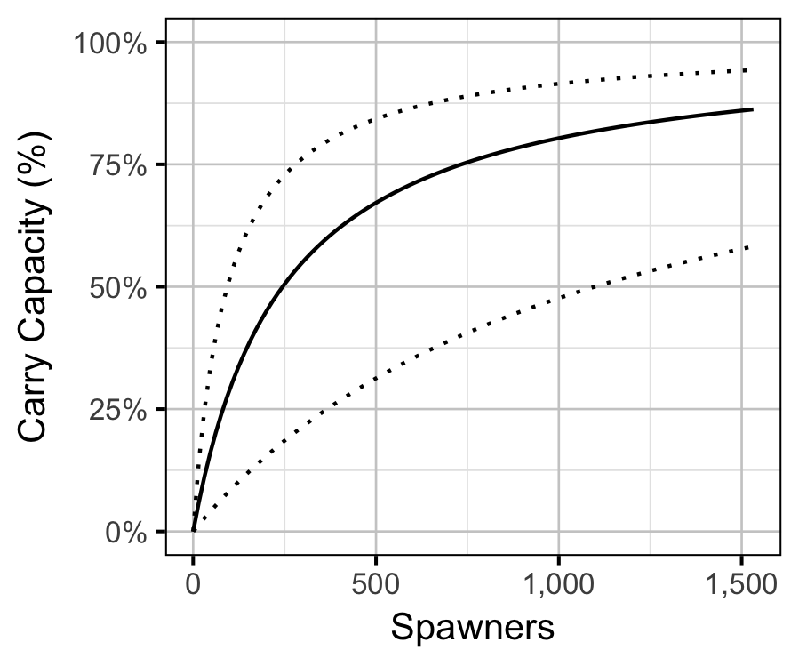
The age-1 carrying capacity (\(K\)) is given by:
\[ K = \frac{a}{b} \quad.\]
Model Templates
Abundance
  data {

    int<lower=0> nMarked;
    int<lower=0> Marked[nMarked];
    int<lower=0> Resighted[nMarked];
    int<lower=0> IndexMarked[nMarked];

    int<lower=0> nObs;
    int Marking[nObs];
    int Index[nObs];
    int<lower=0> nSwimmer;
    int<lower=0> Swimmer[nObs];
    int<lower=0> nYear;
    int<lower=0> Year[nObs];
    real Width[nObs];
    real Rkm[nObs];
    int<lower=0> nSite;
    int<lower=0> Site[nObs];

    real SiteLength[nObs];
    real SurveyProportion[nObs];

    int Count[nObs];
  }
  parameters {
    real bEfficiency;
    real bEfficiencyIndex;

    real bDensity;
    vector[nYear] bDensityYear;
    real bDensityWidth;
    vector[4] bDensityRkm;
    real<lower=0> sDensitySite;
    vector[nSite] bDensitySite;

    real bEfficiencyMarking;
    real bEfficiencyMarkingIndex;

    real<lower=0,upper=5> sEfficiencySwimmer;
    vector[nSwimmer] bEfficiencySwimmer;

    real<lower=0> sDispersion;
  }
  model {

    vector[nObs] eDensity;
    vector[nObs] eEfficiency;
    vector[nObs] eAbundance;
    vector[nObs] eCount;

    sDispersion ~ gamma(0.01, 0.01);

    bDensity ~ normal(0, 2);
    bDensityRkm ~ normal(0, 2);
    sDensitySite ~ uniform(0, 5);
    bDensitySite ~ normal(0, sDensitySite);
    bDensityWidth ~ normal(0, 2);
    bDensityYear ~ normal(0, 5);

    bEfficiency ~ normal(0, 5);
    bEfficiencyIndex ~ normal(0, 5);
    bEfficiencyMarking ~ normal(0, 5);
    bEfficiencyMarkingIndex ~ normal(0, 5);
    sEfficiencySwimmer ~ uniform(0, 5);
    bEfficiencySwimmer ~ normal(0, sEfficiencySwimmer);

    for (i in 1:nMarked) {
      target += binomial_lpmf(Resighted[i] | Marked[i],
        inv_logit(
          bEfficiency +
          bEfficiencyIndex * IndexMarked[i] +
          bEfficiencyMarking +
          bEfficiencyMarkingIndex * IndexMarked[i]
        ));
    }

    for (i in 1:nObs) {
      eDensity[i] = exp(bDensity +
                        bDensityRkm[1] * Rkm[i] +
                        bDensityRkm[2] * pow(Rkm[i], 2.0) +
                        bDensityRkm[3] * pow(Rkm[i], 3.0) +
                        bDensityRkm[4] * pow(Rkm[i], 4.0) +
                        bDensitySite[Site[i]] +
                        bDensityYear[Year[i]] +
                        bDensityWidth * log(Width[i]));

      eEfficiency[i] = inv_logit(
        bEfficiency +
        bEfficiencyIndex * Index[i] +
        bEfficiencyMarking * Marking[i] +
        bEfficiencyMarkingIndex * Index[i] * Marking[i] +
        bEfficiencySwimmer[Swimmer[i]]);

      eAbundance[i] = eDensity[i] * SiteLength[i];

      eCount[i] = eAbundance[i] * eEfficiency[i] * SurveyProportion[i];
    }

    target += neg_binomial_2_lpmf(Count | eCount, sDispersion);
  }
Template 1. Abundance model description.
Stock-Recruitment
model {
  a ~ dnorm(8000 * 0.5^4, 250^-2) T(0, )
  b ~ dunif(0, 0.1)
  sScaling ~ dunif(0, 5)

  eRecruits <- a * Spawners / (1 + Spawners * b)

  for(i in 1:nObs) {
    esRecruits[i] <- SDLogRecruits[i] * sScaling
    Recruits[i] ~ dlnorm(log(eRecruits[i]), esRecruits[i]^-2)
  }
Template 2. Stock-Recruitment model description.
Results
Tables
Abundance
Table 1. Parameter descriptions.
| Parameter | Description |
|---|---|
bDensity |
Intercept for log(eDensity) |
bDensityRkm[x] |
xth-order polynomial coefficients of effect of river kilometer on bDensity |
bDensitySite[i] |
Effect of ith Site on bDensity |
bDensityWidth |
Effect of Width on bDensity |
bDensityYear[i] |
Effect of ith Year on bDensity |
bEfficiency |
Intercept of logit(eEfficiency) |
bEfficiencyIndex |
Effect of Index on bEfficiency |
bEfficiencyMarking |
Effect of Marking on bEfficiency |
bEfficiencyMarkingIndex |
Effect of Marking and Index on bEfficiency |
bEfficiencySwimmer[i] |
Effect of ith Swimmer on bEfficiency |
eAbundance[i] |
Expected abundance of fish at site of ith visit |
eCount[i] |
Expected total number of fish at site of ith visit |
eDensity[i] |
Expected lineal density of fish at site of ith visit |
eEfficiency[i] |
Expected observer efficiency on ith visit |
Index |
Whether the ith visit was to an index site |
Marking[i] |
Whether the ith visit was to a site with marked fish |
Rkm[i] |
River kilometer of ith visit |
sDensitySite |
SD of bDensitySite |
sDispersion |
Overdispersion of Count[i] |
sEfficiencySwimmer |
SD of bEfficiencySwimmer |
Site[i] |
Site of ith visit |
SiteLength[i] |
Length of site of ith visit |
SurveyProportion[i] |
Proportion of site surveyed on ith visit |
Swimmer[i] |
Snorkeler on ith site visit |
Width[i] |
Useable width of site on ith visit |
Year[i] |
Year of ith site visit |
Table 2. Model coefficients.
| term | estimate | sd | zscore | lower | upper | pvalue |
|---|---|---|---|---|---|---|
| bDensity | -0.5609736 | 1.2717405 | -0.4748684 | -3.0208802 | 1.7686930 | 0.6730 |
| bDensityRkm[1] | -0.2245419 | 0.0970234 | -2.3050645 | -0.4188671 | -0.0320095 | 0.0240 |
| bDensityRkm[2] | 0.6614224 | 0.1137607 | 5.8202288 | 0.4212796 | 0.8853642 | 0.0005 |
| bDensityRkm[3] | 0.0309741 | 0.0382207 | 0.8185385 | -0.0419120 | 0.1073823 | 0.4310 |
| bDensityRkm[4] | -0.3002494 | 0.0383004 | -7.8520963 | -0.3760327 | -0.2241509 | 0.0005 |
| bDensityWidth | 0.0816910 | 0.0283956 | 2.8775942 | 0.0254561 | 0.1377320 | 0.0010 |
| bDensityYear[1] | 0.4807932 | 1.2962360 | 0.4227568 | -1.8357639 | 3.0299739 | 0.7250 |
| bDensityYear[2] | -0.3464799 | 1.2935789 | -0.2387211 | -2.6933792 | 2.1272273 | 0.7980 |
| bDensityYear[3] | -0.7047454 | 1.2807716 | -0.4904629 | -3.0051360 | 1.8556464 | 0.6430 |
| bDensityYear[4] | -0.7545865 | 1.2846435 | -0.5454590 | -3.0895398 | 1.7895746 | 0.6050 |
| bDensityYear[5] | -0.3468520 | 1.2966775 | -0.2186230 | -2.6968581 | 2.2429440 | 0.8190 |
| bDensityYear[6] | 0.0395578 | 1.2717297 | 0.0627167 | -2.2843352 | 2.5126749 | 0.9710 |
| bDensityYear[7] | 0.0103889 | 1.2666607 | 0.0462209 | -2.3013677 | 2.4891637 | 0.9930 |
| bDensityYear[8] | -0.3197939 | 1.2688035 | -0.2281621 | -2.6648160 | 2.1053966 | 0.8310 |
| bDensityYear[9] | -0.7803547 | 1.2670294 | -0.5927232 | -3.1533316 | 1.6692387 | 0.5830 |
| bDensityYear[10] | -1.6874992 | 1.2756542 | -1.2863060 | -4.0218208 | 0.7823581 | 0.2100 |
| bDensityYear[11] | -1.2588629 | 1.2687599 | -0.9555919 | -3.6158763 | 1.1808410 | 0.3660 |
| bEfficiency | -1.7819382 | 0.1703980 | -10.4469313 | -2.1061139 | -1.4321656 | 0.0005 |
| bEfficiencyIndex | 0.1934140 | 0.4060052 | 0.4667747 | -0.5683309 | 0.9881197 | 0.6640 |
| bEfficiencyMarking | 0.1022605 | 0.1238488 | 0.7975761 | -0.1474622 | 0.3439068 | 0.4510 |
| bEfficiencyMarkingIndex | 1.9852189 | 0.3887763 | 5.0685101 | 1.2059535 | 2.7109611 | 0.0005 |
| sDensitySite | 0.6598949 | 0.0429870 | 15.3610139 | 0.5757140 | 0.7456404 | 0.0005 |
| sDispersion | 1.1754351 | 0.0673789 | 17.4748628 | 1.0549137 | 1.3210813 | 0.0005 |
| sEfficiencySwimmer | 0.3535370 | 0.1081607 | 3.4335531 | 0.2132199 | 0.6352534 | 0.0005 |
Table 3. Model summary.
| n | K | nsamples | nchains | nsims | rhat | converged |
|---|---|---|---|---|---|---|
| 2916 | 24 | 2000 | 4 | 4000 | 1.01 | TRUE |
Table 4. Summary survey information by year and river.
| Year | River | Sites | SurveyLength | SurveyPercent | Fish | Marked | Resighted |
|---|---|---|---|---|---|---|---|
| 2006 | Duncan | 0 | 0.0 | 0 | 0 | 0 | 0 |
| 2006 | Lardeau | 35 | 2.0 | 1 | 657 | 122 | 79 |
| 2007 | Duncan | 0 | 0.0 | 0 | 0 | 0 | 0 |
| 2007 | Lardeau | 47 | 2.7 | 2 | 260 | 0 | 0 |
| 2008 | Duncan | 0 | 0.0 | 0 | 0 | 0 | 0 |
| 2008 | Lardeau | 97 | 7.5 | 5 | 618 | 94 | 54 |
| 2009 | Duncan | 0 | 0.0 | 0 | 0 | 0 | 0 |
| 2009 | Lardeau | 83 | 5.0 | 4 | 384 | 0 | 0 |
| 2010 | Duncan | 0 | 0.0 | 0 | 0 | 0 | 0 |
| 2010 | Lardeau | 48 | 2.5 | 2 | 307 | 0 | 0 |
| 2011 | Duncan | 32 | 1.8 | 4 | 149 | 0 | 0 |
| 2011 | Lardeau | 264 | 15.8 | 11 | 1947 | 0 | 0 |
| 2012 | Duncan | 71 | 3.8 | 7 | 481 | 0 | 0 |
| 2012 | Lardeau | 257 | 15.2 | 11 | 1691 | 43 | 6 |
| 2013 | Duncan | 117 | 7.0 | 14 | 828 | 56 | 10 |
| 2013 | Lardeau | 308 | 18.0 | 13 | 1236 | 145 | 27 |
| 2014 | Duncan | 77 | 4.9 | 9 | 242 | 70 | 14 |
| 2014 | Lardeau | 273 | 16.2 | 12 | 928 | 96 | 13 |
| 2016 | Duncan | 70 | 3.6 | 7 | 137 | 0 | 0 |
| 2016 | Lardeau | 257 | 14.7 | 10 | 324 | 14 | 2 |
| 2017 | Duncan | 99 | 6.2 | 12 | 250 | 30 | 5 |
| 2017 | Lardeau | 604 | 38.4 | 27 | 1326 | 45 | 1 |
Table 5. Summary survey information by year.
| Year | Sites | SurveyLength | SurveyPercent | Fish | Marked | Resighted |
|---|---|---|---|---|---|---|
| 2006 | 35 | 2.0 | 1 | 657 | 122 | 79 |
| 2007 | 47 | 2.7 | 1 | 260 | 0 | 0 |
| 2008 | 97 | 7.5 | 4 | 618 | 94 | 54 |
| 2009 | 83 | 5.0 | 3 | 384 | 0 | 0 |
| 2010 | 48 | 2.5 | 1 | 307 | 0 | 0 |
| 2011 | 296 | 17.6 | 9 | 2096 | 0 | 0 |
| 2012 | 328 | 19.0 | 10 | 2172 | 43 | 6 |
| 2013 | 425 | 25.0 | 13 | 2064 | 201 | 37 |
| 2014 | 350 | 21.0 | 11 | 1170 | 166 | 27 |
| 2016 | 327 | 18.3 | 10 | 461 | 14 | 2 |
| 2017 | 703 | 44.6 | 23 | 1576 | 75 | 6 |
Stock-Recruitment
Table 6. Parameter descriptions.
| Parameter | Description |
|---|---|
a |
Recruits per Spawner at low density |
b |
Density-dependence |
eRecruits[i] |
Expected number of recruits from ith spawn year |
esRecruits[i] |
Expected SD of residual variation in Recruits |
Recruits[i] |
Number of recruits from ith spawn year |
SDLogRecruits[i] |
Standard deviation of uncertainty in log(Recruits[i]) |
Spawners[i] |
Number of spawners in ith spawn year |
sScaling |
Scaling term for SD of residual variation in log(eRecruits) |
Table 7. Model coefficients.
| term | estimate | sd | zscore | lower | upper | pvalue |
|---|---|---|---|---|---|---|
| a | 481.4567932 | 200.8357326 | 2.520724 | 203.6611240 | 944.6992620 | 5e-04 |
| b | 0.0040898 | 0.0026784 | 1.705611 | 0.0009107 | 0.0107306 | 5e-04 |
| sScaling | 2.3845734 | 0.6332814 | 3.909790 | 1.5157516 | 4.0364412 | 5e-04 |
Table 8. Model summary.
| n | K | nsamples | nchains | nsims | rhat | converged |
|---|---|---|---|---|---|---|
| 11 | 3 | 2000 | 4 | 4e+05 | 1 | TRUE |
Table 9. Estimated carry capacity.
| estimate | sd | zscore | lower | upper |
|---|---|---|---|---|
| 120849.6 | 48569.61 | 2.660642 | 70856.94 | 234359.9 |
Figures
Abundance
Stock-Recruitment
Recommendations
- Scan and add all field cards to database.
- Add all GPS tracks to database.
- Verify reorganised data.
- Estimate observer fry length cutoffs based on length-frequency distributions.
- Account for spatial autocorrelation in density estimates.
- Use WAIC to estimate predictive value of habitat variables.
Acknowledgements
The organisations and individuals whose contributions have made this analysis report possible include:
- Habitat Conservation Trust Foundation (HCTF) and the anglers, hunters, trappers and guides who contribute to the Trust.
- Fish and Wildlife Compensation Program (FWCP) and its program partners BC Hydro, the Province of BC and Fisheries and Oceans Canada.
- Ministry of Forests, Lands and Natural Resource
Operations (MFLNRO)
- Greg Andrusak
- Gary Pavan
- Stefan Himmer
- Vicky Lipinski
- John Hagen
- Scott Decker
- Jody Schick
- Gillian Sanders
- Jeremy Baxter
- Jeff Berdusco
- Dave Derosa
- Seb Dalgarno