Curtis and Qua Creeks Productivity Analysis 2018
The suggested citation for this analytic report is:
Thorley, J.L. and Dalgarno, S. (2019) Curtis and Qua Creeks Productivity Analysis 2018. A Poisson Consulting Analysis Report. URL: https://www.poissonconsulting.ca/f/1060059151.
Background
Invertebrate and fish data were collected from Curtis and Qua Creeks from 2015 to 2017, water chemistry data were collected from 2015 to 2018, and periphyton data were collected in 2015, 2016 and 2018 to assess their productivity. The fish data were collected by depletion electrofishing.
Methods
Data Collection
The data were collected by the Salmo Streamkeepers and Poisson Consulting in 2015 and by the Salmo Streamkeepers from 2016 to 2018. The invertebrate data were processed by Westcott Environmental Services and the water chemistry and periphyton data by CARO Analytic. The data were provided to Poisson in the form of an Excel database.
Data Preparation
The data were manipulated using R version 3.5.2 (R Core Team 2015) and imported into an SQLite database.
Statistical Analysis
Model parameters were estimated using Bayesian methods. The Bayesian estimates were produced using JAGS (Plummer 2003). For additional information on Bayesian estimation the reader is referred to McElreath (2016).
Unless indicated otherwise, the Bayesian analyses used uninformative normal prior distributions (Kery and Schaub 2011, 36). The posterior distributions were estimated from 1500 Markov Chain Monte Carlo (MCMC) samples thinned from the second halves of 3 chains (Kery and Schaub 2011, 38–40). Model convergence was confirmed by ensuring that \(\hat{R} \leq 1.1\) (Kery and Schaub 2011, 40) and \(\textrm{ESS} \geq 150\) for each of the monitored parameters (Kery and Schaub 2011, 61). Where \(\hat{R}\) is the potential scale reduction factor and \(\textrm{ESS}\) is the effective sample size.
The parameters are summarised in terms of the point estimate, standard deviation (sd), the z-score, lower and upper 95% confidence/credible limits (CLs) and the p-value (Kery and Schaub 2011, 37, 42). The estimate is the median (50th percentile) of the MCMC samples, the z-score is \(\mathrm{mean}/\mathrm{sd}\) and the 95% CLs are the 2.5th and 97.5th percentiles. A p-value of 0.05 indicates that the lower or upper 95% CL is 0.
Where informative, model adequacy was confirmed by examination of residual plots for the full model(s).
The results are displayed graphically by plotting the modeled relationships between particular variables and the response(s) with the remaining variables held constant. In general, continuous and discrete fixed variables are held constant at their mean and first level values, respectively, while random variables are held constant at their typical values (expected values of the underlying hyperdistributions) (Kery and Schaub 2011, 77–82). When informative the influence of particular variables is expressed in terms of the effect size (i.e., percent change in the response variable) with 95% confidence/credible intervals (CIs, Bradford, Korman, and Higgins 2005).
The analyses were implemented using R version 3.5.2
(R Core Team 2015) and the
mbr family of packages.
Model Descriptions
Periphyton Growth
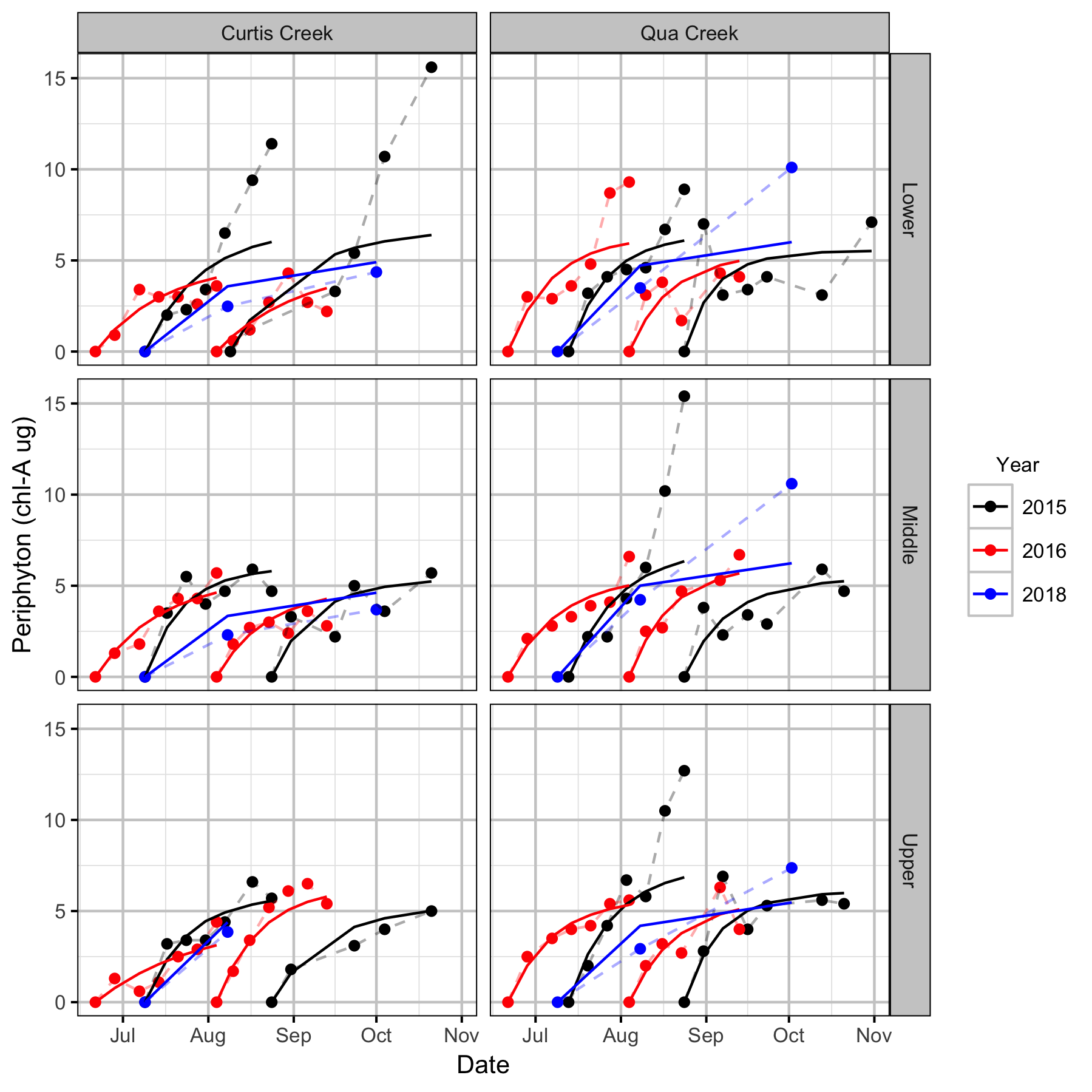
Periphyton growth can be modelled using sigmoidal curves (Rodriguez 1987). Here we use the flexible unified-Richards model (Tjørve and Tjørve 2010)
\[P_t = A(1 + (d - 1)\exp(-K(t - T_i)/d^{d/(1-d)}))^{1/(1-d)}\] to model the periphyton density at time \(t\) (\(P_t\)) where \(A\) is the maximum density, \(K\) is the maximum relative growth rate, \(T_i\) is the time at maximum growth, and \(d\) is the relative value at maximum growth (Tjørve and Tjørve 2010).
Key assumptions of the growth model include:
- \(A\) can vary randomly by series within location within creek within year
- \(K\) can vary randomly by series within location within creek within year
- \(T_i\) is 0
- \(d\) is 0
- The residual variation in \(P_t\) is log-normally distributed.
Rainbow Trout Density
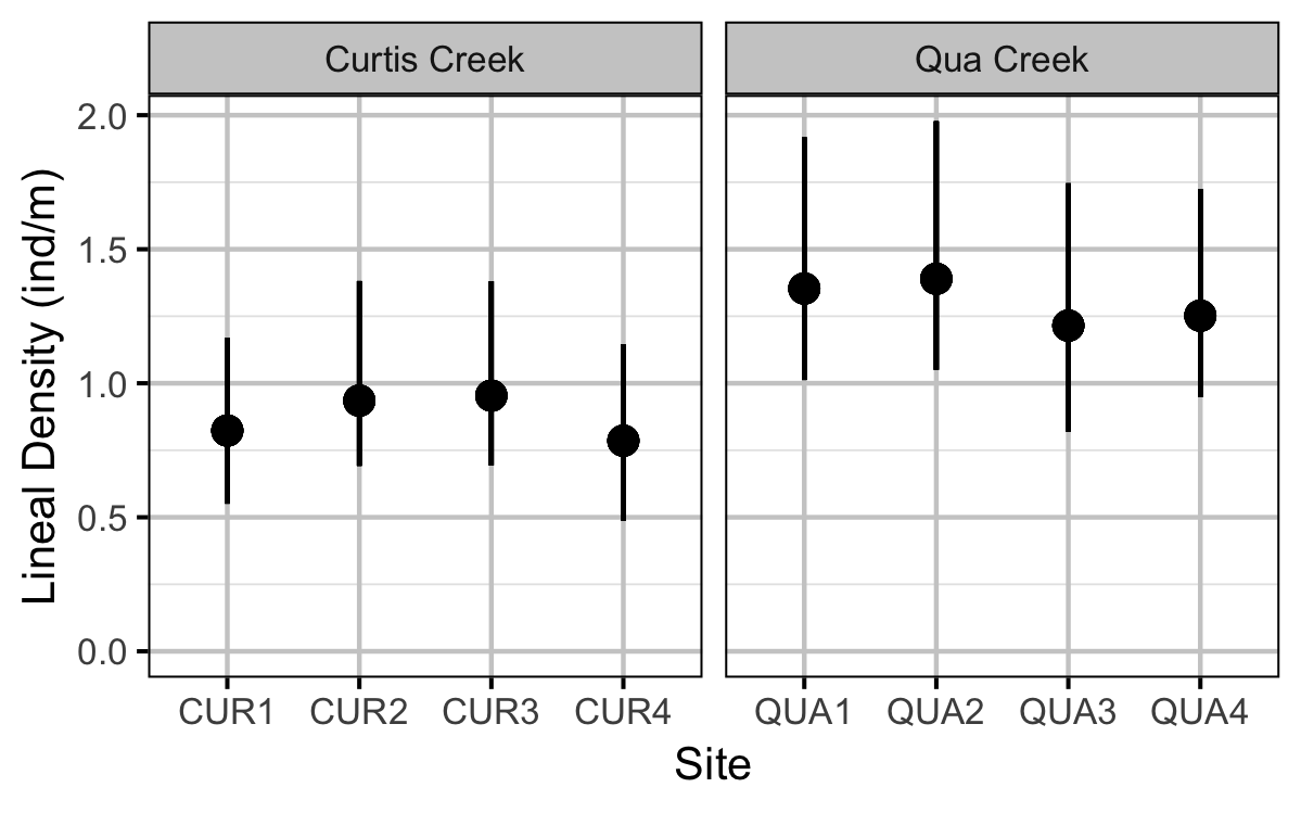
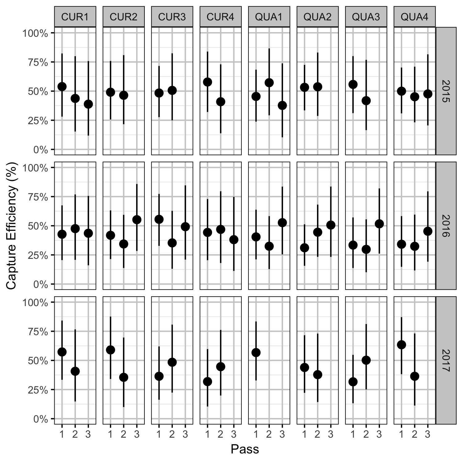
The density of Rainbow Trout each site was estimated using a removal model (Wyatt 2002).
Key assumptions of the removal model include:
- Lineal density varies by creek and randomly by site.
- Capture efficiency varies randomly by pass within site within year.
- The number of fish caught on each pass is binomially distributed.
Preliminary analyses indicated that year was not a significant predictor of density.
Model Templates
Periphyton Growth
model{
  bA ~ dnorm(0, 5^-2)
  bK ~ dnorm(-5, 5^-2)

  sAYearCreekLocationSeries ~ dunif(0, 1)
  sKYearCreekLocationSeries ~ dunif(0, 1)
  for(i in 1:nYear) {
    for(j in 1:nCreek) {
      for(k in 1:nLocation) {
        for(l in 1:nSeries) {
          bAYearCreekLocationSeries[i, j, k, l] ~ dnorm(0, sAYearCreekLocationSeries^-2)
          bKYearCreekLocationSeries[i, j, k, l] ~ dnorm(0, sKYearCreekLocationSeries^-2)
        }
      }
    }
  }

  sPeriphyton ~ dunif(0, 1)
  for (i in 1:length(Periphyton)) {
    log(eA[i]) <- bA +  bAYearCreekLocationSeries[Year[i],Creek[i],Location[i],Series[i]]
    log(eK[i]) <- bK +  bKYearCreekLocationSeries[Year[i],Creek[i],Location[i],Series[i]]
    ePeriphyton[i] <- eA[i] * (1 - exp(-eK[i] * Days[i]))
    Periphyton[i] ~ dlnorm(log(ePeriphyton[i]), sPeriphyton^-2)
  }
..
Template 1. The model description.
Rainbow Trout Density
model{
  bDensity ~ dnorm(0, 5^-2)

  bDensityCreek[1] <- 0
  for (i in 2:nCreek) {
    bDensityCreek[i] ~ dnorm(0, 5^-2)
  }

  sDensitySite ~ dunif(0, 5)
  for (i in 1:nSite) {
    bDensitySite[i] ~ dnorm(0, sDensitySite^-2)
  }

  bEfficiency ~ dnorm(0, 2^-2)

  sEfficiencyYearSitePass ~ dunif(0, 2)
  for(i in 1:nYear) {
    for(j in 1:nSite) {
      for(k in 1:nPass) {
        bEfficiencyYearSitePass[i,j,k] ~ dnorm(0, sEfficiencyYearSitePass^-2)
      }
    }
  }

  for (i in 1:length(SiteLength)) {
    log(eDensity[i]) <- bDensity + bDensityCreek[Creek[i]] + bDensitySite[Site[i]]
    eAbundance[i] ~ dpois(eDensity[i] * SiteLength[i])
    eRemaining[i,1] <- eAbundance[i]

    for(j in 1:nPass) {
      logit(eEfficiency[i,j]) <- bEfficiency + bEfficiencyYearSitePass[Year[i], Site[i], j]
      Catch[i,j] ~ dbin(eEfficiency[i,j], eRemaining[i,j])
      eRemaining[i,j+1] <- eRemaining[i,j] - Catch[i,j]
    }
  }
..
Template 2. The model description.
Results
Tables
Periphyton Growth
Table 1. Parameter descriptions.
| Parameter | Description |
|---|---|
bA |
Intercept for eA |
bAYearCreekLocationSeries[i,j,k,l] |
Effect of ith year at jth creek at
kth location at lth series on bA |
bK |
Intercept for eK |
bKYearCreekLocationSeries[i,j,k,l] |
Effect of ith year at jth creek at
kth location at lth series on bK |
Days[i] |
Time since deployment in creek at ith
observation (days) |
eA[i] |
Expected maximum ePeriphyton for ith
observation |
eK[i] |
Expected maximum relative growth of ePeriphyton
for ith observation |
ePeriphyton[i] |
Expected Periphyton for ith observation |
Periphyton[i] |
Measured Chlorophyll-A density at ith
observation (mg/m2) |
sAYearCreekLocationSeries |
SD of bAYearCreekLocationSeries |
sKYearCreekLocationSeries |
SD of bKYearCreekLocationSeries |
sPeriphyton |
SD of residual variation in Periphyton |
Table 2. Model coefficients.
| term | estimate | sd | zscore | lower | upper | pvalue |
|---|---|---|---|---|---|---|
| bA | 1.7587003 | 0.0902420 | 19.493587 | 1.5857452 | 1.9494140 | 7e-04 |
| bK | -2.8978879 | 0.1948726 | -14.883883 | -3.2791066 | -2.4978765 | 7e-04 |
| sAYearCreekLocationSeries | 0.2089841 | 0.0838858 | 2.441237 | 0.0325656 | 0.3746033 | 7e-04 |
| sKYearCreekLocationSeries | 0.4524928 | 0.1709028 | 2.640269 | 0.0718987 | 0.7893817 | 7e-04 |
| sPeriphyton | 0.3694194 | 0.0279164 | 13.234978 | 0.3152628 | 0.4257058 | 7e-04 |
Table 3. Model summary.
| n | K | nchains | niters | nthin | ess | rhat | converged |
|---|---|---|---|---|---|---|---|
| 148 | 5 | 3 | 500 | 100 | 906 | 1.006 | TRUE |
Rainbow Trout Density
Table 4. Parameter descriptions.
| Parameter | Description |
|---|---|
bDensity |
Intercept for log(eDensity) |
bDensityCreek[i] |
Effect of ith Creek on bDensity |
bDensitySite[i] |
Effect of ith Site on bDensity |
bEfficiency |
Intercept for logit(eEfficiency) |
bEfficiencyYearSitePass[i,j,k] |
Effect of ith Year at jth Site at
kth Pass on bEfficiency |
Catch[i, j] |
Catch on jth pass at ith site visit |
Creek |
Creek on ith site visit |
eAbundance[i] |
Expected total number of fish at ith site
visit |
eDensity[i] |
Expected lineal density at ith site visit
(fish/m) |
eEfficiency[i] |
Expected efficiency during ith site visit |
eRemaining[i, j] |
Expected number of fish remaining after jth
pass at ith site visit |
sDensitySite |
SD of bDensitySite |
sEfficiencyYearSitePass |
SD of bEfficiencyYearSitePass |
Site |
Site on ith site visit |
SiteLength |
Length of creek surveyed during ith site
visit (m) |
Year |
Year on ith site visit |
Table 5. Model coefficients.
| term | estimate | sd | zscore | lower | upper | pvalue |
|---|---|---|---|---|---|---|
| bDensity | -0.1348905 | 0.1850769 | -0.7735391 | -0.5433389 | 0.2076869 | 0.3760 |
| bDensityCreek[2] | 0.4019674 | 0.2094297 | 1.8869675 | -0.0220680 | 0.7745569 | 0.0600 |
| bEfficiency | -0.1838870 | 0.3138420 | -0.6294796 | -0.8744477 | 0.3715226 | 0.5613 |
| sDensitySite | 0.1477767 | 0.1682751 | 1.1043174 | 0.0056875 | 0.6336051 | 0.0007 |
| sEfficiencyYearSitePass | 0.6501171 | 0.2028888 | 3.2307456 | 0.2761678 | 1.0674429 | 0.0007 |
Table 6. Model summary.
| n | K | nchains | niters | nthin | ess | rhat | converged |
|---|---|---|---|---|---|---|---|
| 58 | 5 | 3 | 500 | 10 | 178 | 1.024 | TRUE |
Bull Trout
Table 7. Bull Trout captured during electrofishing surveys.
| Waterbody | Dayte | Year | EFSite | Location | Species | ForkLength | BodyWeight |
|---|---|---|---|---|---|---|---|
| Curtis Creek | 1972-08-03 | 2016 | CUR1 | 1 | BT | 91 | 10 |
| Curtis Creek | 1972-08-03 | 2016 | CUR1 | 1 | BT | 95 | 10 |
| Curtis Creek | 1972-08-03 | 2016 | CUR2 | 2 | BT | 92 | 10 |
| Curtis Creek | 1972-08-14 | 2017 | CUR2 | 2 | BT | 115 | 18 |
Figures
Water Temperature
Periphyton Growth
Benthic Invertebrates
Rainbow Trout Length-Weight
Rainbow Trout Density
Chemical
Acknowledgements
The organisations and individuals whose contributions have made this analysis report possible include:
- Fish and Wildlife Compensation Program
- Crystal Klym
- Poisson Consulting
- Robyn Irvine
- Salmo Streamkeepers
- Gerry Nellestin
- Eleanor Duifhuis
- Tanya Chi Tran
- Westcott Environmental Services
- Lynn Westcott
References
Bradford, Michael J, Josh Korman, and Paul S Higgins. 2005. “Using Confidence Intervals to Estimate the Response of Salmon Populations (Oncorhynchus Spp.) to Experimental Habitat Alterations.” Canadian Journal of Fisheries and Aquatic Sciences 62 (12): 2716–26. https://doi.org/10.1139/f05-179.
Kery, Marc, and Michael Schaub. 2011. Bayesian Population Analysis Using WinBUGS : A Hierarchical Perspective. Boston: Academic Press. http://www.vogelwarte.ch/bpa.html.
McElreath, Richard. 2016. Statistical Rethinking: A Bayesian Course with Examples in R and Stan. Chapman & Hall/CRC Texts in Statistical Science Series 122. Boca Raton: CRC Press/Taylor & Francis Group.
Plummer, Martyn. 2003. “JAGS: A Program for Analysis of Bayesian Graphical Models Using Gibbs Sampling.” In Proceedings of the 3rd International Workshop on Distributed Statistical Computing (DSC 2003), edited by Kurt Hornik, Friedrich Leisch, and Achim Zeileis. Vienna, Austria.
R Core Team. 2015. “R: A Language and Environment for Statistical Computing.” Vienna, Austria: R Foundation for Statistical Computing. http://www.R-project.org/.
Rodriguez, Marco A. 1987. “Estimating Periphyton Growth Parameters Using Simple Models.” Limnology and Oceanography 32 (2): 458–64.
Tjørve, Even, and Kathleen M. C. Tjørve. 2010. “A Unified Approach to the Richards-Model Family for Use in Growth Analyses: Why We Need Only Two Model Forms.” Journal of Theoretical Biology 267 (3): 417–25. https://doi.org/10.1016/j.jtbi.2010.09.008.
Wyatt, Robin J. 2002. “Estimating Riverine Fish Population Size from Single- and Multiple-Pass Removal Sampling Using a Hierarchical Model.” Canadian Journal of Fisheries and Aquatic Sciences 59 (4): 695–706. https://doi.org/10.1139/f02-041.