Alouette Reservoir Kokanee Size-at-Age 2019
The suggested citation for this analytic appendix is:
Thorley, J.L. (2020) Alouette Reservoir Kokanee Size-at-Age 2019. A Poisson Consulting Analytic Appendix. URL: https://www.poissonconsulting.ca/f/1304398440.
Background
The Kokanee age structure population analysis (ALUMON #6) is a multi-year study to address potential impacts of reservoir operations on the reservoirs’ kokanee (Oncorhynchus nerka) population (Andrusak 2016).
The management question addressed in the current analysis is whether:
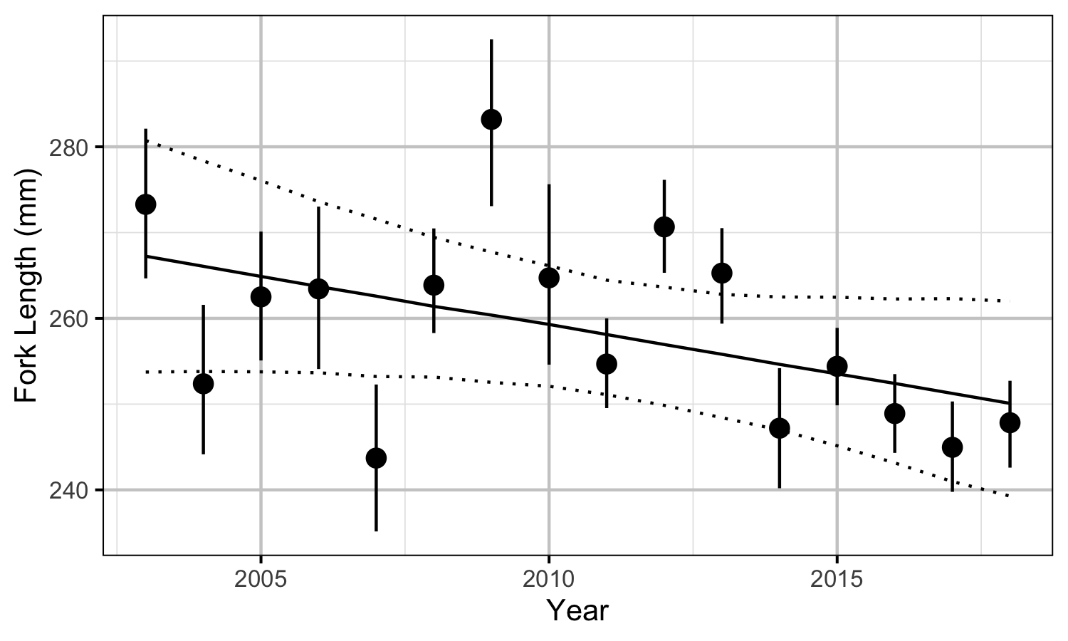
- The size-at-age of the kokanee population remains stable, or decreases with time once the standing crop has stabilized with the annual addition of fertilizer.
Methods
Data Preparation
The gillnetting and productivity data were provided by BC Ministry of Forests, Lands and Natural Resource Operations.
Size-at-Age
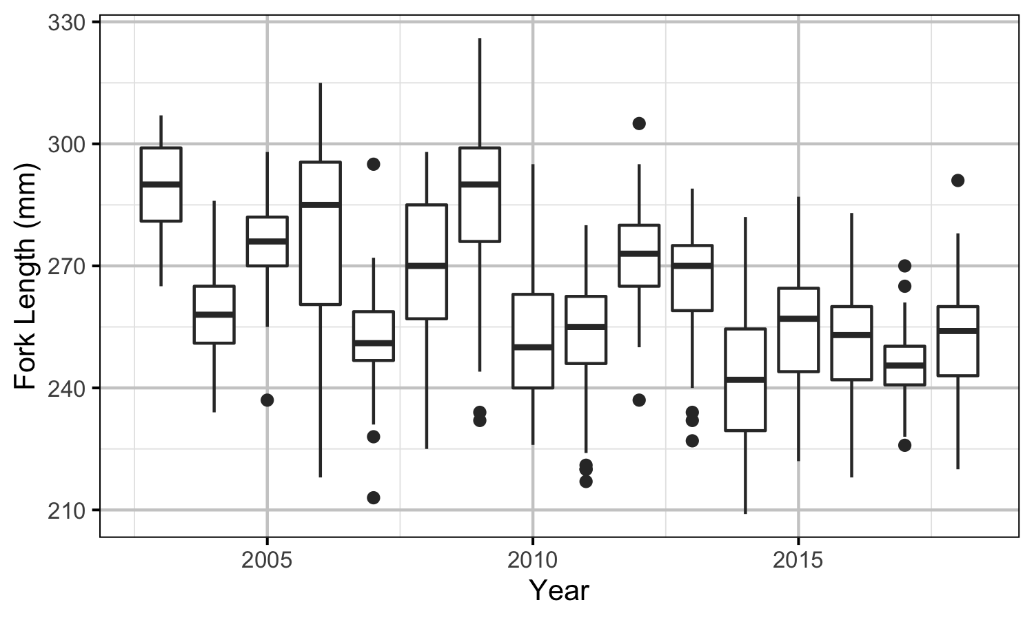
The data used for size-at-age analysis were the lengths of age-3 Kokanee caught during gillnetting surveys.
During the survey data preparation it was assumed that:
- Standing crop stabilized in 2003.
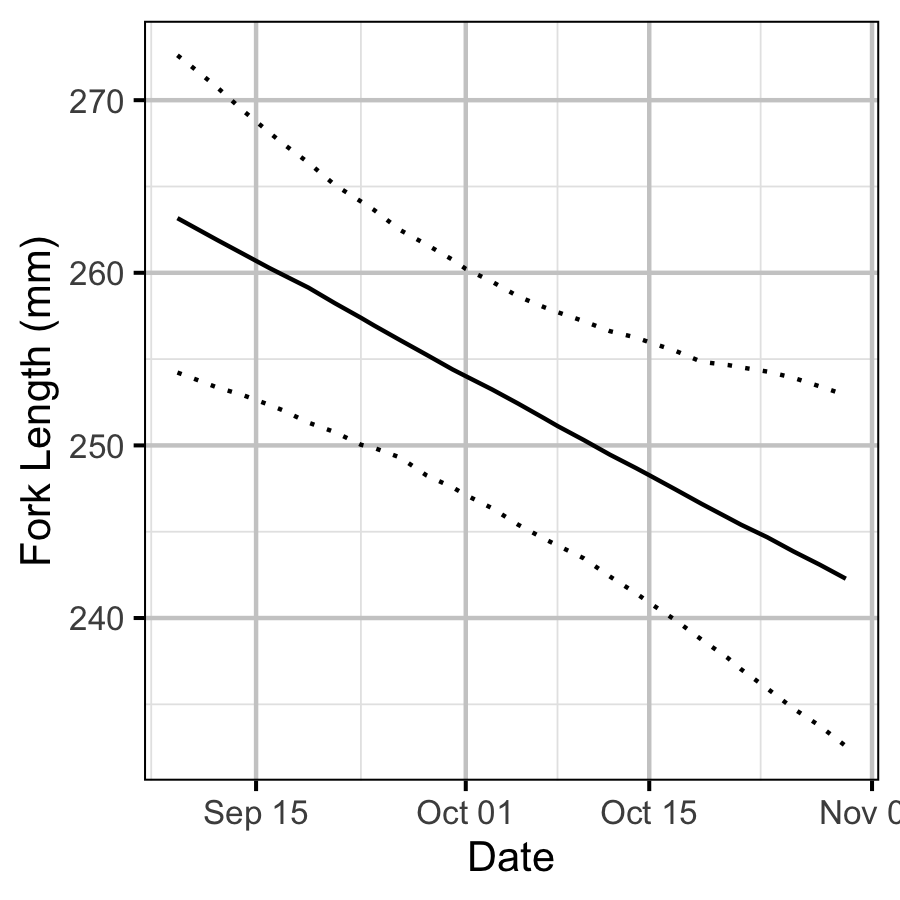
- Only fish that were netted in September and October had indicative lengths.
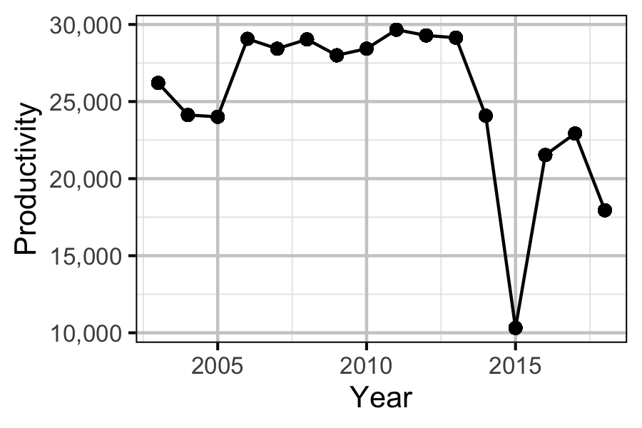
- The productivity was the N:P ratio from 2008-2013 of 7.45 multiplied by the nutrient with the lower value in the ratio (P).
Statistical Analysis
Model parameters were estimated using Bayesian methods. The estimates were produced using JAGS (Plummer 2015). For additional information on Bayesian estimation the reader is referred to McElreath (2016).
Unless stated otherwise, the Bayesian analyses used weakly informative normal and half-normal prior distributions (Gelman, Simpson, and Betancourt 2017). The posterior distributions were estimated from 1500 Markov Chain Monte Carlo (MCMC) samples thinned from the second halves of 3 chains (Kery and Schaub 2011, 38–40). Model convergence was confirmed by ensuring that the potential scale reduction factor \(\hat{R} \leq 1.05\) (Kery and Schaub 2011, 40) and the effective sample size (Brooks et al. 2011) \(\textrm{ESS} \geq 150\) for each of the monitored parameters (Kery and Schaub 2011, 61).
The parameters are summarised in terms of the point estimate, standard deviation (sd), the z-score, lower and upper 95% confidence/credible limits (CLs) and the p-value (Kery and Schaub 2011, 37, 42). The estimate is the median (50th percentile) of the MCMC samples, the z-score is \(\mathrm{mean}/\mathrm{sd}\) and the 95% CLs are the 2.5th and 97.5th percentiles. A p-value of 0.05 indicates that the lower or upper 95% CL is 0.
The results are displayed graphically by plotting the modeled relationships between particular variables and the response(s) with the remaining variables held constant. In general, continuous and discrete fixed variables are held constant at their mean and first level values, respectively, while random variables are held constant at their typical values (expected values of the underlying hyperdistributions) (Kery and Schaub 2011, 77–82). When informative the influence of particular variables is expressed in terms of the effect size (i.e., percent change in the response variable) with 95% confidence/credible intervals (CIs, Bradford, Korman, and Higgins 2005).
The analyses were implemented using R version 3.6.2
(R Core Team 2019) and the
mbr family of packages.
Model Descriptions
Size-at-Age
The fork length of age-3 Kokanee was analysed using a hierarchical Bayesian generalized mixed effects model.
Key assumptions of the model include:
- Length varies with year and day of the year.
- Length varies randomly with year and location within year.
- The residual variation in length is log-normally distributed.
Preliminary analysis indicated that productivity and type of net set were not significant predictors of the length of age-3 Kokanee.
Model Templates
Size-at-Age
.model{
  bLength ~ dnorm(5, 1^-2)
  bYear ~ dnorm(0, 1^-2)
  bDayte ~ dnorm(0, 1^-2)

  bHabitat[1] <- 0
  for (i in 2:nHabitat) {
      bHabitat[i] ~ dnorm(0, 1^-2)
  }

  sLengthAnnual ~ dnorm(0, 1^-2) T(0,)
  for (i in 1:nAnnual) {
      bAnnual[i] ~ dnorm(0, sLengthAnnual^-2)
  }

  sLocationAnnual ~ dnorm(0, 1^-2) T(0,)
  for (i in 1:nLocation) {
    for(j in 1:nAnnual) {
      bLocationAnnual[i, j] ~ dnorm(0, sLocationAnnual^-2)
    }
  }

  sLength ~ dnorm(0, 1^-2) T(0,)

  for(i in 1:length(Length)){
    log(eLength[i]) <- bLength + bHabitat[Habitat[i]] + bYear * Year[i] + bDayte * Dayte[i] + bAnnual[Annual[i]] + bLocationAnnual[Location[i], Annual[i]]

    Length[i] ~ dlnorm(log(eLength[i]), sLength^-2)
  }
..
Block 1. Model description.
Results
Tables
Size-at-Age
Table 1. Parameter descriptions.
| Parameter | Description |
|---|---|
Annual[i] |
Year of capture of ith fish (as a discrete variable) |
bAnnual[i] |
Effect of ith Annual on bLength |
bDayte |
Effect of Dayte on bLength |
bHabitat |
Effect of Habitat on bLength |
bLength |
Intercept for log(eLength) |
bLocationAnnual[i, j] |
Effect of ith Location in jth Annual on bLength |
bYear |
Effect of Year on bLength |
Dayte[i] |
Day of the year of capture of ith fish |
eLength[i] |
Expected Length of ith fish |
Habitat[i] |
Habitat of capture of ith fish (Pelagic vs Nearshore) |
Length[i] |
Measured fork length of ith fish |
Location[i] |
Location of capture of ith fish |
sLength |
SD of residual variation in Length about log(eLength) |
sLengthAnnual |
SD of bAnnual |
sLocationAnnual |
SD of bLocationAnnual |
Year[i] |
Year of capture of ith fish (as a continuous variable) |
Table 2. Model coefficients.
| term | estimate | sd | zscore | lower | upper | pvalue |
|---|---|---|---|---|---|---|
| bDayte | -0.0016044 | 0.0005773 | -2.790751 | -0.0026885 | -0.0004505 | 0.0053 |
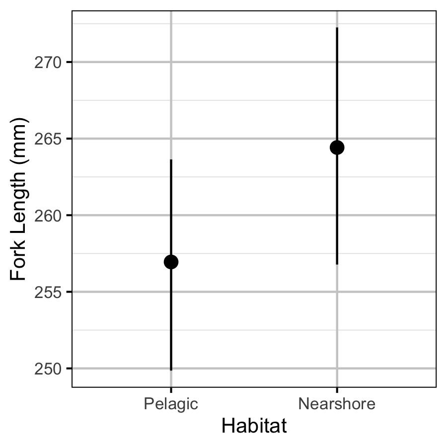
| bHabitat[2] | 0.0286835 | 0.0126052 | 2.316889 | 0.0050427 | 0.0540167 | 0.0187 |
| bLength | 5.5484459 | 0.0133073 | 416.914040 | 5.5206369 | 5.5739654 | 0.0007 |
| bYear | -0.0044153 | 0.0026635 | -1.648343 | -0.0094982 | 0.0010432 | 0.1053 |
| sLength | 0.0515231 | 0.0011101 | 46.465559 | 0.0495159 | 0.0539029 | 0.0007 |
| sLengthAnnual | 0.0446892 | 0.0107811 | 4.294392 | 0.0297489 | 0.0718660 | 0.0007 |
| sLocationAnnual | 0.0188552 | 0.0034137 | 5.585832 | 0.0129948 | 0.0262084 | 0.0007 |
Table 3. Model summary.
| n | K | nchains | niters | nthin | ess | rhat | converged |
|---|---|---|---|---|---|---|---|
| 1136 | 7 | 3 | 500 | 50 | 286 | 1.004 | TRUE |
Figures
Size-at-Age
Acknowledgements
The organisations and individuals whose contributions have made this analysis report possible include:
- Ministry of Forests, Lands and Natural Resource Operations (MFLNRO)
- Jen Sarchuk
- Shannon Harris
- Greg Andrusak
- Redfish Consulting
- Harvey Andrusak
- Poisson Consulting
- Robyn Irvine
- Mauricio Campos
- Patrick Hogan
References
Andrusak, G. F. 2016. “Alouette Kokanee Age Structure Analysis (ALUMON#6)-2014.” A Redfish Consulting Ltd. Report. Vancouver, BC: Ministry of Environment.
Bradford, Michael J, Josh Korman, and Paul S Higgins. 2005. “Using Confidence Intervals to Estimate the Response of Salmon Populations (Oncorhynchus Spp.) to Experimental Habitat Alterations.” Canadian Journal of Fisheries and Aquatic Sciences 62 (12): 2716–26. https://doi.org/10.1139/f05-179.
Brooks, Steve, Andrew Gelman, Galin L. Jones, and Xiao-Li Meng, eds. 2011. Handbook for Markov Chain Monte Carlo. Boca Raton: Taylor & Francis.
Gelman, Andrew, Daniel Simpson, and Michael Betancourt. 2017. “The Prior Can Often Only Be Understood in the Context of the Likelihood.” Entropy 19 (10): 555. https://doi.org/10.3390/e19100555.
Kery, Marc, and Michael Schaub. 2011. Bayesian Population Analysis Using WinBUGS : A Hierarchical Perspective. Boston: Academic Press. http://www.vogelwarte.ch/bpa.html.
McElreath, Richard. 2016. Statistical Rethinking: A Bayesian Course with Examples in R and Stan. Chapman & Hall/CRC Texts in Statistical Science Series 122. Boca Raton: CRC Press/Taylor & Francis Group.
Plummer, Martyn. 2015. “JAGS Version 4.0.1 User Manual.” http://sourceforge.net/projects/mcmc-jags/files/Manuals/4.x/.
R Core Team. 2019. R: A Language and Environment for Statistical Computing. Vienna, Austria: R Foundation for Statistical Computing. https://www.R-project.org/.